CS 3343 Analysis of Algorithms Lecture 22 Minimum


 – V: a set of vertices –")


. Output: a MST T. Randomly")
. Output: a MST T. Randomly select a")

![Idea 2: distance array // For each vertex v, d[v] is the min distance](https://slidetodoc.com/presentation_image/6beb237a2e5e4f71e84db25fb7f575f7/image-34.jpg "Idea 2: distance array // For each vertex v, d[v] is the min distance")


![Time complexity? // For each vertex v, d[v] is the min distance from v](https://slidetodoc.com/presentation_image/6beb237a2e5e4f71e84db25fb7f575f7/image-49.jpg "Time complexity? // For each vertex v, d[v] is the min distance from v")
 • Observation – In idea 2, we need to")


![Complete Prim’s Algorithm MST-Prim(G, w, r) Q = V[G]; for each u Q Overall](https://slidetodoc.com/presentation_image/6beb237a2e5e4f71e84db25fb7f575f7/image-66.jpg "Complete Prim’s Algorithm MST-Prim(G, w, r) Q = V[G]; for each u Q Overall")


 – Possibly Θ(m + n log")
- Slides: 94
CS 3343: Analysis of Algorithms Lecture 22: Minimum Spanning Tree
Outline • Review of last lecture • Prim’s algorithm and Kruskal’s algorithm for MST in detail
Graph Review • G = (V, E) – V: a set of vertices – E: a set of edges – Degree: number of edges • In-degree vs out-degree • Types of graphs – – Directed / undirected Weighted / un-weighted Dense / sparse Connected / disconnected
Graph representations • Adjacency matrix 1 2 4 3 A 1 2 3 4 1 0 1 1 0 2 0 0 1 0 3 0 0 4 0 0 1 0 How much storage does the adjacency matrix require? A: O(V 2)
Graph representations • Adjacency list 1 2 3 3 2 4 3 3 How much storage does the adjacency list require? A: O(V+E)
Graph representations • Undirected graph 1 2 4 3 2 3 1 2 3 4 A 1 2 0 1 1 0 3 1 1 4 0 0 3 4 1 1 0 0 0 1 1 0
Graph representations • Weighted graph A 1 2 3 4 1 5 6 2 9 4 4 3 1 0 5 6 0 2, 5 3, 6 1, 5 3, 9 1, 6 2, 9 3, 4 2 5 0 9 0 4, 4 3 6 9 0 4 4 0 0 4 0
Analysis of time complexity • Convention: – Number of vertices: n, |V|, V – Number of edges: m, |E|, E – O(V+E) is the same as O(n+m) or O(|V|+|E|)
Tradeoffs between the two representations |V| = n, |E| = m Adj Matrix test (u, v) E Θ(1) Degree(u) Θ(n) Memory Θ(n 2) Edge insertion Θ(1) Edge deletion Θ(1) Graph traversal Θ(n 2) Adj List O(n) Θ(n+m) Θ(1) O(n) Θ(n+m) Both representations are very useful and have different properties, although adjacency lists are probably better for most problems
Minimum Spanning Tree • Problem: given a connected, undirected, weighted graph: 6 4 5 14 9 2 10 15 3 8
Minimum Spanning Tree • Problem: given a connected, undirected, weighted graph, find a spanning tree using edges that minimize the total weight 6 4 5 14 9 2 10 15 3 8 • A spanning tree is a tree that connects all vertices • Number of edges = ? • A spanning tree has no designated root.
Minimum Spanning Tree • MSTs satisfy the optimal substructure property: an optimal tree is composed of optimal subtrees – Let T be an MST of G with an edge (u, v) in the middle – Removing (u, v) partitions T into two trees T 1 and T 2 – w(T) = w(u, v) + w(T 1) + w(T 2) • Claim 1: T 1 is an MST of G 1 = (V 1, E 1), and T 2 is an MST of G 2 = (V 2, E 2) T 2 T 1 ’ u v Proof by contradiction: • if T 1 is not optimal, we can replace T 1 with a better spanning tree, T 1’ • T 1’, T 2 and (u, v) form a new spanning tree T’ • W(T’) < W(T). Contradiction.
Minimum Spanning Tree • MSTs satisfy the optimal substructure property: an optimal tree is composed of optimal subtrees – Let T be an MST of G with an edge (u, v) in the middle – Removing (u, v) partitions T into two trees T 1 and T 2 – w(T) = w(u, v) + w(T 1) + w(T 2) • Claim 2: (u, v) is the lightest edge connecting G 1 = (V 1, E 1) and G 2 = (V 2, E 2) T 2 T 1 x u v y Proof by contradiction: • if (u, v) is not the lightest edge, we can remove it, and reconnect T 1 and T 2 with a lighter edge (x, y) • T 1, T 2 and (x, y) form a new spanning tree T’ • W(T’) < W(T). Contradiction.
Algorithms • Generic idea: – Compute MSTs for sub-graphs – Connect two MSTs for sub-graphs with the lightest edge • Two of the most well-known algorithms – Prim’s algorithm – Kruskal’s algorithm – Let’s first talk about the ideas behind the algorithms without worrying about the implementation and analysis
Prim’s algorithm • Basic idea: – Start from an arbitrary single node • A MST for a single node has no edge – Gradually build up a single larger and larger MST 6 7 5 Not yet discovered Fully explored nodes Discovered but not fully explored nodes
Prim’s algorithm • Basic idea: – Start from an arbitrary single node • A MST for a single node has no edge – Gradually build up a single larger and larger MST 6 7 2 5 9 4 Not yet discovered Fully explored nodes Discovered but not fully explored nodes
Prim’s algorithm • Basic idea: – Start from an arbitrary single node • A MST for a single node has no edge – Gradually build up a single larger and larger MST 6 7 2 5 9 4
Prim’s algorithm in words • Randomly pick a vertex as the initial tree T • Gradually expand into a MST: – For each vertex that is not in T but directly connected to some nodes in T • Compute its minimum distance to any vertex in T – Select the vertex that is closest to T • Add it to T
Example a 6 12 5 b 14 7 8 c 3 f e d 10 9 15 g h
Example a 6 12 5 b 14 7 8 c 3 f e d 10 9 15 g h
Example a 6 12 5 b 14 7 8 c 3 f e d 10 9 15 g h
Example a 6 12 5 b 14 7 8 c 3 f e d 10 9 15 g h
Example a 6 12 5 b 14 7 8 c 3 f e d 10 9 15 g h
Example a 6 12 5 b 14 7 8 c 3 f e d 10 9 15 g h
Example a 6 12 5 b 14 7 8 c 3 f e d 10 9 15 g h
Example a 6 12 5 b 14 7 8 c 3 f e d 10 9 15 g h
Example a 6 12 5 b 14 7 8 c 3 f e d 10 9 15 g h
Example a 6 12 5 b 14 7 8 c 3 f e d 10 9 15 g h
Example a 6 12 5 b 14 7 8 c 3 f e d 10 9 15 g h
Example a 6 12 5 b 14 7 8 c 3 f e d 10 9 15 g h
Pseudocode for Prim’s algorithm Given G = (V, E). Output: a MST T. Randomly select a vertex v S = {v}; A = V S; T = {}. While (A is not empty) find a vertex u A that connects to vertex v S such that w(u, v) ≤ w(x, y), for any x A and y S S = S U {u}; A = A {u}; T = T U (u, v). End Return T
Time complexity Given G = (V, E). Output: a MST T. Randomly select a vertex v S = {v}; A = V S; T = {}. n vertices While (A is not empty) find a vertex u A that connects to vertex v S such that w(u, v) ≤ w(x, y), for any x A and y S S = S U {u}; A = A {u}; T = T U (u, v). End Return T Time complexity: n * (time spent on purple line per vertex) • Naïve: test all edges => Θ(n * m) • Improve: keep the list of candidates in an array => Θ(n 2) • Better: with priority queue => Θ(m log n)
Idea 1: naive find a vertex u A that connects to vertex v S such that w(u, v) ≤ w(x, y), for any x A and y S min_weight = infinity. For each edge (x, y) E if x A, y S, and w(x, y) < min_weight u = x; v = y; min_weight = w(x, y); time spent per vertex: Θ(m) Total time complexity: Θ(n*m)
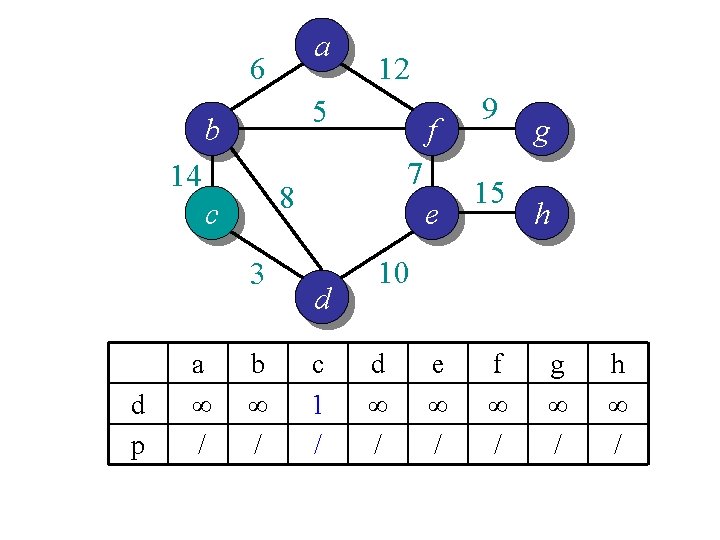
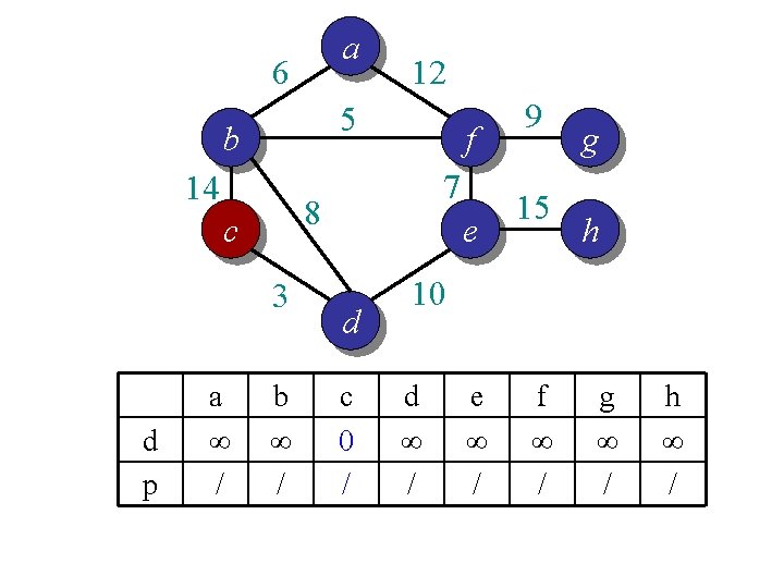
Idea 2: distance array // For each vertex v, d[v] is the min distance from v to any node already in S // p[v] is the parent node of v in the spanning tree For each v V d[v] = infinity; p[v] = null; Randomly select a v, d[v] = 1; // d[v]=1 just to ensure proper start S = {}; A = V; T = {}. While (A is not empty) Search d to find the smallest d[u] > 0. S = S U {u}; A = A {u}; T = T U (u, p[u]); d[u] = 0. For each v in adj[u] if d[v] > w(u, v) d[v] = w(u, v); p[v] = u; End
a 6 5 b Discovered 14 3 d p a ∞ / f 7 8 c Explored 12 b 14 c e d c 0 / 9 15 10 d 3 c g h Not discovered e ∞ / f ∞ / g ∞ / h ∞ /
a 6 5 b 14 3 d p f 7 8 c a ∞ / 12 b 14 c e d c 0 / 9 15 g h 10 d 0 c e ∞ / f ∞ / g ∞ / h ∞ /
a 6 5 b 14 3 d p f 7 8 c a ∞ / 12 b 8 d e d c 0 / 9 15 g h 10 d 0 c e 10 d f ∞ / g ∞ / h ∞ /
a 6 5 b 14 3 d p f 7 8 c a ∞ / 12 b 0 d e d c 0 / 9 15 g h 10 d 0 c e 10 d f ∞ / g ∞ / h ∞ /
a 6 5 b 14 3 d p f 7 8 c a 6 b 12 b 0 d e d c 0 / 9 15 g h 10 d 0 c e 10 d f 5 b g ∞ / h ∞ /
a 6 5 b 14 3 d p f 7 8 c a 6 b 12 b 0 d e d c 0 / 9 15 g h 10 d 0 c e 10 d f 0 b g ∞ / h ∞ /
a 6 5 b 14 3 d p f 7 8 c a 6 b 12 b 0 d e d c 0 / 9 15 g h 10 d 0 c e 7 f f 0 b g 9 f h ∞ /
a 6 5 b 14 3 d p f 7 8 c a 0 b 12 b 0 d e d c 0 / 9 15 g h 10 d 0 c e 7 f f 0 b g 9 f h ∞ /
a 6 5 b 14 3 d p f 7 8 c a 0 b 12 b 0 d e d c 0 / 9 15 g h 10 d 0 c e 0 f f 0 b g 9 f h ∞ /
a 6 5 b 14 3 d p f 7 8 c a 0 b 12 b 0 d e d c 0 / 9 15 g h 10 d 0 c e 0 f f 0 b g 9 f h 15 e
a 6 5 b 14 3 d p f 7 8 c a 0 b 12 b 0 d e d c 0 / 9 15 g h 10 d 0 c e 0 f f 0 b g 0 f h 15 e
a 6 5 b 14 3 d p f 7 8 c a 0 b 12 b 0 d e d c 0 / 9 15 g h 10 d 0 c e 0 f f 0 b g 0 f h 0 e
Time complexity? // For each vertex v, d[v] is the min distance from v to any node already in S // p[v] is the parent node of v in the spanning tree For each v V d[v] = infinity; p[v] = null; Randomly select a v, d[v] = 1; // d[v]=1 just to ensure proper start S = {}. T = {}. A = V. n vertices While (A is not empty) Θ(n) per vertex Search d to find the smallest d[u] > 0. S = S U {u}; A = A {u}; T = T U (u, p[u]); d[u] = 0. O(n) per vertex if using adj list For each v in adj[u] (n) per vertex if using adj matrix if d[v] > w(u, v) d[v] = w(u, v); p[v] = u; End Overall complexity: Θ (n 2)
Idea 3: priority queue (min-heap) • Observation – In idea 2, we need to search the distance array n times, each time we only look for the minimum element. – Distance array size = n – n x n = n 2 • Can we do better? – Priority queue (heap) enables fast retrieval of min (or max) elements – log (n) for most operations
Example a 6 12 5 b 14 f 7 8 c 3 e 9 15 g h 10 d a b c d e f g h ∞ ∞ ∞ ∞
Example a 6 12 5 b 14 f 7 8 c 3 e 15 g h 10 d Change. Key 9 c b a d e f g h 0 ∞ ∞ ∞ ∞
Example a 6 12 5 b 14 f 7 8 c 3 e 15 10 d Exctract. Min 9 h b a d e f g ∞ ∞ ∞ ∞ g h
Example a 6 12 5 b 14 f 7 8 c 3 e 9 15 10 d Change. Key d b a h e f g 3 14 ∞ ∞ ∞ g h
Example a 6 5 b 14 f 7 8 c 3 e 10 d Exctract. Min b 12 g a h e f 14 ∞ ∞ ∞ 9 15 g h
Example a 6 12 5 b 14 f 7 8 c 3 Changekey e d 10 b e a h g f 8 10 ∞ ∞ 9 15 g h
Example a 6 12 5 b 14 f 7 8 c 3 e d 10 Extract. Min e f 10 ∞ a h g ∞ ∞ ∞ 9 15 g h
Example a 6 12 5 b 14 f 7 8 c 3 e 10 d Changekey f e a h g 5 10 6 ∞ ∞ 9 15 g h
Example a 6 12 5 b 14 f 7 8 c 3 e 10 d Extract. Min a e g h 6 10 ∞ ∞ 9 15 g h
Example a 6 12 5 b 14 f 7 8 c 3 e 10 d Changekey a e g h 6 7 9 ∞ 9 15 g h
Example a 6 12 5 b 14 7 8 c 3 f e d Extract. Min e h g 7 ∞ 9 10 9 15 g h
Example a 6 12 5 b 14 7 8 c 3 Extract. Min g h 9 ∞ f e d 10 9 15 g h
Example a 6 12 5 b 14 7 8 c 3 e d Changekey g h 9 15 f 10 9 15 g h
Example a 6 12 5 b 14 7 8 c 3 Extract. Min h 15 f e d 10 9 15 g h
Example a 6 12 5 b 14 7 8 c 3 f e d 10 9 15 g h
Complete Prim’s Algorithm MST-Prim(G, w, r) Q = V[G]; for each u Q Overall running time: Θ(m log n) key[u] = ; p[u] = null; Cost per Change. Key key[r] = 0; n vertices while (Q not empty) u = Extract. Min(Q); Θ(n) times for each v Adj[u] if (v Q and w(u, v) < key[v]) p[v] = u; Change. Key(v, w(u, v)); Θ(n 2) times? How often is Extract. Min() called? How often is Change. Key() called? Θ(m) times (with adj list)
Kruskal’s algorithm in words • Procedure: – Sort all edges into non-decreasing order – Initially each node is in its own tree – For each edge in the sorted list • If the edge connects two separate trees, then – join the two trees together with that edge
c-d: 3 b-f: 5 b-a: 6 f-e: 7 b-d: 8 f-g: 9 d-e: 10 a-f: 12 b-c: 14 e-h: 15 Example a 6 12 5 b 14 7 8 c 3 f e d 10 9 15 g h
c-d: 3 b-f: 5 b-a: 6 f-e: 7 b-d: 8 f-g: 9 d-e: 10 a-f: 12 b-c: 14 e-h: 15 Example a 6 12 5 b 14 7 8 c 3 f e d 10 9 15 g h
c-d: 3 b-f: 5 b-a: 6 f-e: 7 b-d: 8 f-g: 9 d-e: 10 a-f: 12 b-c: 14 e-h: 15 Example a 6 12 5 b 14 7 8 c 3 f e d 10 9 15 g h
c-d: 3 b-f: 5 b-a: 6 f-e: 7 b-d: 8 f-g: 9 d-e: 10 a-f: 12 b-c: 14 e-h: 15 Example a 6 12 5 b 14 7 8 c 3 f e d 10 9 15 g h
c-d: 3 b-f: 5 b-a: 6 f-e: 7 b-d: 8 f-g: 9 d-e: 10 a-f: 12 b-c: 14 e-h: 15 Example a 6 12 5 b 14 7 8 c 3 f e d 10 9 15 g h
c-d: 3 b-f: 5 b-a: 6 f-e: 7 b-d: 8 f-g: 9 d-e: 10 a-f: 12 b-c: 14 e-h: 15 Example a 6 12 5 b 14 7 8 c 3 f e d 10 9 15 g h
c-d: 3 b-f: 5 b-a: 6 f-e: 7 b-d: 8 f-g: 9 d-e: 10 a-f: 12 b-c: 14 e-h: 15 Example a 6 12 5 b 14 7 8 c 3 f e d 10 9 15 g h
c-d: 3 b-f: 5 b-a: 6 f-e: 7 b-d: 8 f-g: 9 d-e: 10 a-f: 12 b-c: 14 e-h: 15 Example a 6 12 5 b 14 7 8 c 3 f e d 10 9 15 g h
c-d: 3 b-f: 5 b-a: 6 f-e: 7 b-d: 8 f-g: 9 d-e: 10 a-f: 12 b-c: 14 e-h: 15 Example a 6 12 5 b 14 7 8 c 3 f e d 10 9 15 g h
c-d: 3 b-f: 5 b-a: 6 f-e: 7 b-d: 8 f-g: 9 d-e: 10 a-f: 12 b-c: 14 e-h: 15 Example a 6 12 5 b 14 7 8 c 3 f e d 10 9 15 g h
c-d: 3 b-f: 5 b-a: 6 f-e: 7 b-d: 8 f-g: 9 d-e: 10 a-f: 12 b-c: 14 e-h: 15 Example a 6 12 5 b 14 7 8 c 3 f e d 10 9 15 g h
Time complexity • Depend on implementation • Pseudocode sort all edges according to weights T = {}. tree(v) = v for all v. m edges for each edge (u, v) if tree(u) != tree(v) T = T U (u, v); m times union (tree(u), tree(v)) Θ(m log m) = Θ(m log n) (n-1) times. Overall time complexity: m log n + m t + n u tree union Naïve: Θ(nm) tree finding Better implementation: Θ(m log n)
Disjoint Set Union • Use a linked list to represent tree elements, with pointers back to root: – tree[u] != tree[v]: O(1) – Union(tree[u], tree[v]): “Copy” elements of A into set B by adjusting elements of A to point to B – Each union may take O(n) time – Precisely n-1 unions – O(n 2)?
Disjoint Set Union • Better strategy and analysis – Always copy smaller list into larger list – Size of combined list is at least twice the size of smaller list – Each vertex copied at most logn times before a single tree emerges – Total number of copy operations for n vertex is therefore O(n log n) • Overall time complexity: m log n + m t + n u – t: time for finding tree root is constant – u: time for n union operations is at most nlog (n) – m log n + m t + n u = Θ (m log n + m + n log n) = Θ (m log n) • Conclusion – Kruskal’s algorithm runs in Θ(m log n) for both dense and sparse graph
Example with disjoint set union c-d: 3 b-f: 5 b-a: 6 f-e: 7 b-d: 8 f-g: 9 d-e: 10 a-f: 12 b-c: 14 e-h: 15 a 6 5 b 14 3 b 9 f 7 8 c a 12 15 e h 10 d c g d e f g h
Example with disjoint set union c-d: 3 b-f: 5 b-a: 6 f-e: 7 b-d: 8 f-g: 9 d-e: 10 a-f: 12 b-c: 14 e-h: 15 a 6 5 b 14 3 b 9 f 7 8 c a 12 15 e h 10 d c g d e f g h
Example with disjoint set union c-d: 3 b-f: 5 b-a: 6 f-e: 7 b-d: 8 f-g: 9 d-e: 10 a-f: 12 b-c: 14 e-h: 15 a 6 5 b 14 3 b 9 f 7 8 c a 12 15 e h 10 d f g c d e g h
Example with disjoint set union c-d: 3 b-f: 5 b-a: 6 f-e: 7 b-d: 8 f-g: 9 d-e: 10 a-f: 12 b-c: 14 e-h: 15 a 6 5 b 14 3 f 9 f 7 8 c b 12 15 e h 10 d a g c d e g h
Example with disjoint set union c-d: 3 b-f: 5 b-a: 6 f-e: 7 b-d: 8 f-g: 9 d-e: 10 a-f: 12 b-c: 14 e-h: 15 a 6 5 b 14 3 f 9 f 7 8 c b 12 15 e h 10 d e g a c d g h
Example with disjoint set union c-d: 3 b-f: 5 b-a: 6 f-e: 7 b-d: 8 f-g: 9 d-e: 10 a-f: 12 b-c: 14 e-h: 15 a 6 5 b 14 3 c 9 f 7 8 c b 12 15 e h 10 d d g f e a g h
Example with disjoint set union c-d: 3 b-f: 5 b-a: 6 f-e: 7 b-d: 8 f-g: 9 d-e: 10 a-f: 12 b-c: 14 e-h: 15 a 6 5 b 14 3 c 9 f 7 8 c b 12 15 e h 10 d d g f g e a h
Example with disjoint set union c-d: 3 b-f: 5 b-a: 6 f-e: 7 b-d: 8 f-g: 9 d-e: 10 a-f: 12 b-c: 14 e-h: 15 a 6 5 b 14 3 c 9 f 7 8 c b 12 15 e h 10 d d g f g e a h
Example with disjoint set union c-d: 3 b-f: 5 b-a: 6 f-e: 7 b-d: 8 f-g: 9 d-e: 10 a-f: 12 b-c: 14 e-h: 15 a 6 5 b 14 3 c 9 f 7 8 c b 12 15 e h 10 d d g f g e a h
Example with disjoint set union c-d: 3 b-f: 5 b-a: 6 f-e: 7 b-d: 8 f-g: 9 d-e: 10 a-f: 12 b-c: 14 e-h: 15 a 6 5 b 14 3 c 9 f 7 8 c b 12 15 e h 10 d d g f g e a h
Example with disjoint set union c-d: 3 b-f: 5 b-a: 6 f-e: 7 b-d: 8 f-g: 9 d-e: 10 a-f: 12 b-c: 14 e-h: 15 a 6 5 b 14 3 c 9 f 7 8 c b 12 15 e h 10 d d g f g e h a
Disjoint Set Union • Better strategy and analysis – – Always copy smaller list into larger list Size of combined list is at least twice the size of smaller list Each vertex copied at most logn times before a single tree emerges Total number of copy operations for n vertex is therefore O(n log n) • Overall time complexity: m log n + m t + n u – t: time for finding tree root is constant – u: time for n union operations is at most nlog (n) – m log n + m t + n u = Θ (m log n + m + n log n) = Θ (m log n) • Conclusion – Kruskal’s algorithm runs in Θ(m log n) for both dense and sparse graph • How about using counting sort? – Θ(m + n log n)
Summary • Kruskal’s algorithm – Θ(m log n) – Possibly Θ(m + n log n) with counting sort • Prim’s algorithm – With priority queue : Θ(m log n) • Assume graph represented by adj list – With distance array : Θ(n^2) • Adj list or adj matrix – For sparse graphs priority queue wins – For dense graphs distance array may be better