CS 3343 Analysis of Algorithms Lecture 23 Single

CS 3343: Analysis of Algorithms Lecture 23: Single source shortest path problem

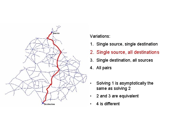
Variations: 1. Single source, single destination 2. Single source, all destinations 3. Single destination, all sources 4. All pairs • Solving 1 is asymptotically the same as solving 2 • 2 and 3 are equivalent • 4 is different

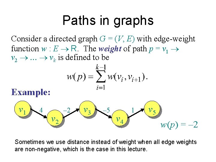
Paths in graphs Consider a directed graph G = (V, E) with edge-weight function w : E R. The weight of path p = v 1 v 2 . . . vk is defined to be . Example: v 1 4 v 2 – 2 v 3 – 5 v 4 1 v 5 w(p) = – 2 Sometimes we use distance instead of weight when all edge weights are non-negative, which is the case in this lecture.

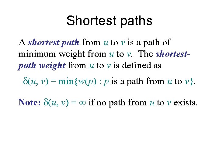
Shortest paths A shortest path from u to v is a path of minimum weight from u to v. The shortestpath weight from u to v is defined as d(u, v) = min{w(p) : p is a path from u to v}. Note: d(u, v) = ¥ if no path from u to v exists.

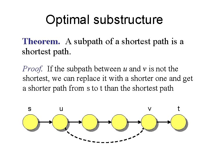
Optimal substructure Theorem. A subpath of a shortest path is a shortest path. Proof. If the subpath between u and v is not the shortest, we can replace it with a shorter one and get a shorter path from s to t than the shortest path s u v t

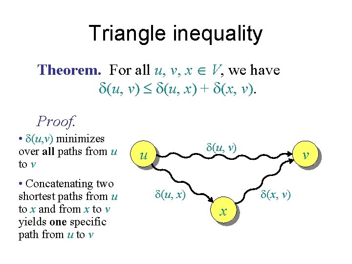
Triangle inequality Theorem. For all u, v, x Î V, we have d(u, v) £ d(u, x) + d(x, v). Proof. • d(u, v) minimizes over all paths from u to v • Concatenating two shortest paths from u to x and from x to v yields one specific path from u to v d(u, v) u d(u, x) v d(x, v) x

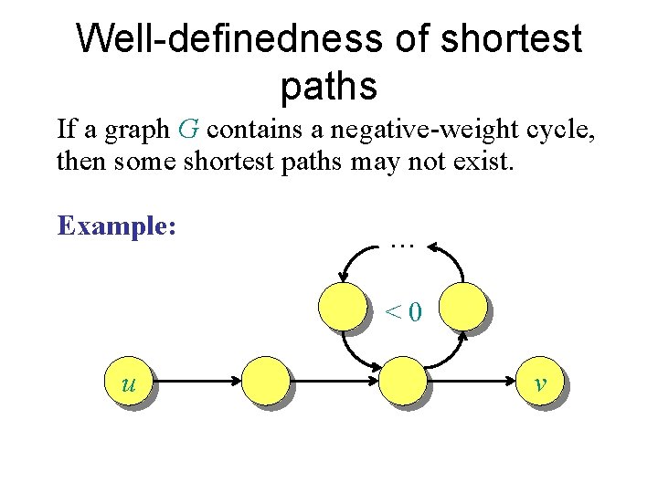
Well-definedness of shortest paths If a graph G contains a negative-weight cycle, then some shortest paths may not exist. Example: … <0 u v

Single-source shortest paths Problem. From a given source vertex s Î V, find the shortest-path weights d(s, v) for all v Î V. If all edge weights w(u, v) are nonnegative, all shortest-path weights must exist.

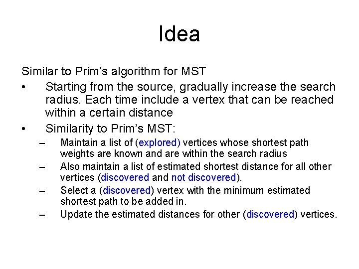
Idea Similar to Prim’s algorithm for MST • Starting from the source, gradually increase the search radius. Each time include a vertex that can be reached within a certain distance • Similarity to Prim’s MST: – – Maintain a list of (explored) vertices whose shortest path weights are known and are within the search radius Also maintain a list of estimated shortest distance for all other vertices (discovered and not discovered). Select a (discovered) vertex with the minimum estimated shortest path to be added in. Update the estimated distances for other (discovered) vertices.

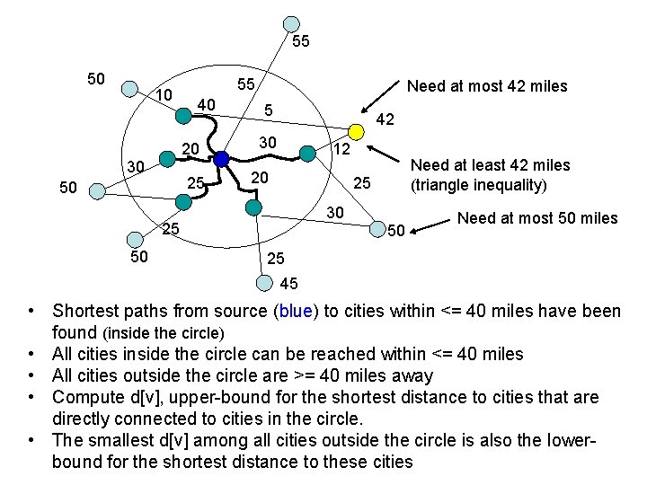
55 50 10 55 40 20 30 25 50 Need at most 42 miles 5 42 30 12 20 25 30 25 50 Need at least 42 miles (triangle inequality) 50 Need at most 50 miles 25 45 • Shortest paths from source (blue) to cities within <= 40 miles have been found (inside the circle) • All cities inside the circle can be reached within <= 40 miles • All cities outside the circle are >= 40 miles away • Compute d[v], upper-bound for the shortest distance to cities that are directly connected to cities in the circle. • The smallest d[v] among all cities outside the circle is also the lowerbound for the shortest distance to these cities

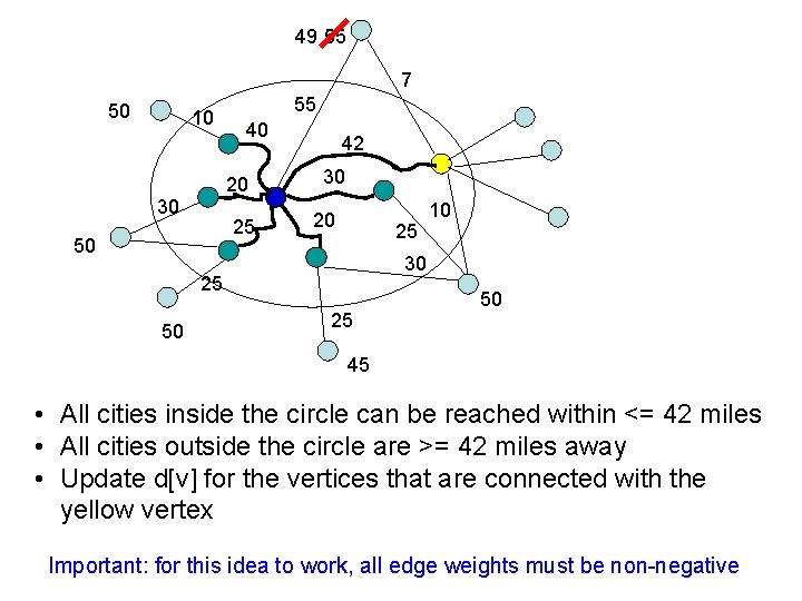
49 55 7 50 10 55 40 20 30 25 50 42 30 20 25 30 25 50 10 25 50 45 • All cities inside the circle can be reached within <= 42 miles • All cities outside the circle are >= 42 miles away • Update d[v] for the vertices that are connected with the yellow vertex Important: for this idea to work, all edge weights must be non-negative

Dijkstra’s algorithm d[v] = ¥ for all v Î V ⊳ d: shortest path length d[s] = 0 ⊳ s: source S= ⊳ set of explored nodes Q = V ⊳ Q: a priority queue maintaining unexplored nodes while Q ¹ do u = Extract. Min (Q) ⊳ u: node to be explored S = S È {u} for each v Î Adj[u] do relaxation if d[v] > d[u] + w(u, v) then change. Key(v, d[u] + w(u, v)) step P[v] = u Remember predecessor on path

Q=V PRIM’s algorithm key[v] = ¥ for all v Î V key[r] = 0 for some arbitrary r Î V Dijkstra’s algorithm d[v] = ¥ for all v Î Vwhile Q ¹ d[s] = 0 u Extract. Min(Q) S= for each v Î Adj[u] Q=V if v Î Q and key[v] > w(u, v) Change. Key(v, w(u, v)) P[v] = u; while Q ¹ do u = Extract. Min (Q) It suffices to only check v Î Q, S = S È {u} but it doesn’t hurt to check all v for each v Î Adj[u] do relaxation if d[v] > d[u] + w(u, v) then change. Key(v, d[u] + w(u, v)) step P[v] = u Remember path

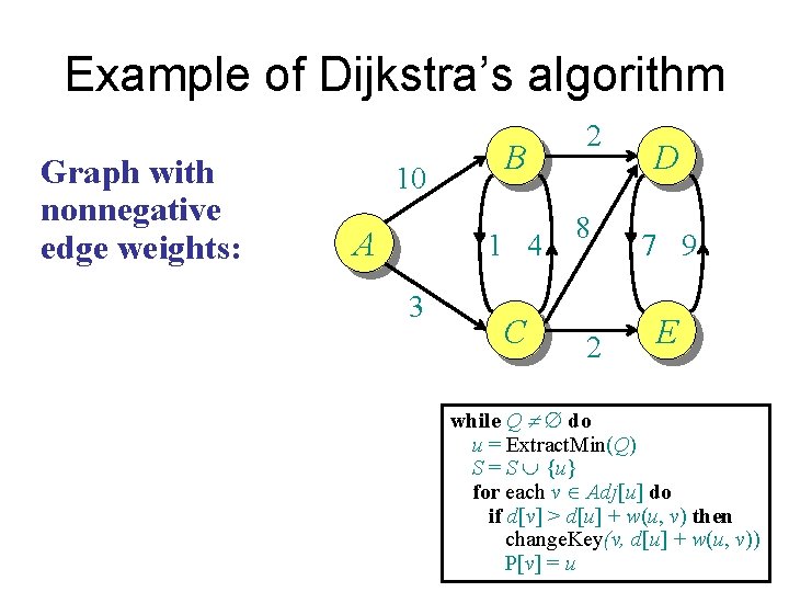
Example of Dijkstra’s algorithm Graph with nonnegative edge weights: 10 A B 1 4 3 C 2 8 2 D 7 9 E while Q ¹ do u = Extract. Min(Q) S = S È {u} for each v Î Adj[u] do if d[v] > d[u] + w(u, v) then change. Key(v, d[u] + w(u, v)) P[v] = u

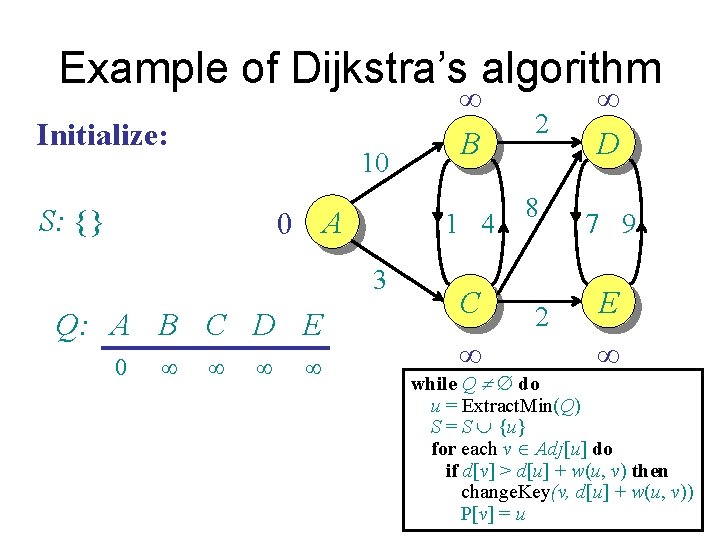
Example of Dijkstra’s algorithm Initialize: 10 S: {} 0 A 1 4 3 Q: A B C D E 0 ¥ ¥ ¥ B C ¥ 2 8 2 ¥ D 7 9 E ¥ while Q ¹ do u = Extract. Min(Q) S = S È {u} for each v Î Adj[u] do if d[v] > d[u] + w(u, v) then change. Key(v, d[u] + w(u, v)) P[v] = u

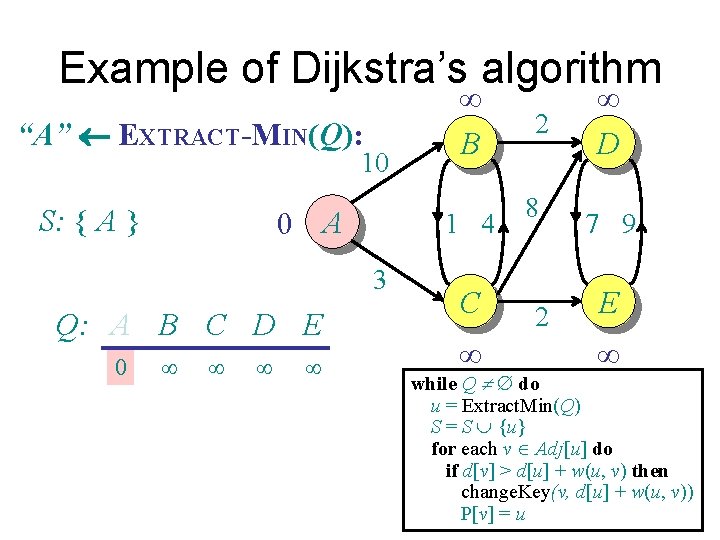
Example of Dijkstra’s algorithm “A” EXTRACT-MIN(Q): 10 S: { A } 0 A 1 4 3 Q: A B C D E 0 ¥ ¥ ¥ B C ¥ 2 8 2 ¥ D 7 9 E ¥ while Q ¹ do u = Extract. Min(Q) S = S È {u} for each v Î Adj[u] do if d[v] > d[u] + w(u, v) then change. Key(v, d[u] + w(u, v)) P[v] = u

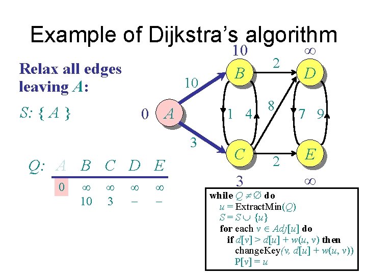
Example of Dijkstra’s algorithm Relax all edges leaving A: 10 S: { A } 0 A 1 4 3 Q: A B C D E 0 ¥ 10 ¥ 3 ¥ - 10 B C 3 2 8 2 ¥ D 7 9 E ¥ while Q ¹ do u = Extract. Min(Q) S = S È {u} for each v Î Adj[u] do if d[v] > d[u] + w(u, v) then change. Key(v, d[u] + w(u, v)) P[v] = u

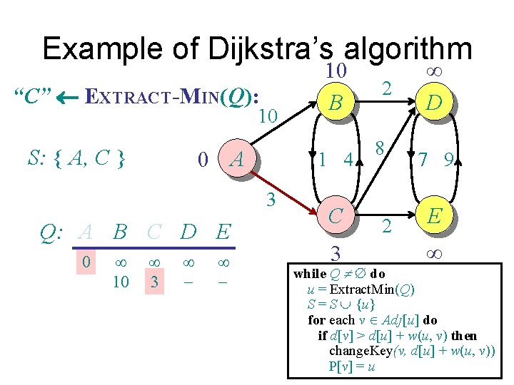
Example of Dijkstra’s algorithm “C” EXTRACT-MIN(Q): 10 S: { A, C } 0 A 1 4 3 Q: A B C D E 0 ¥ 10 ¥ 3 ¥ - 10 B C 3 2 8 2 ¥ D 7 9 E ¥ while Q ¹ do u = Extract. Min(Q) S = S È {u} for each v Î Adj[u] do if d[v] > d[u] + w(u, v) then change. Key(v, d[u] + w(u, v)) P[v] = u

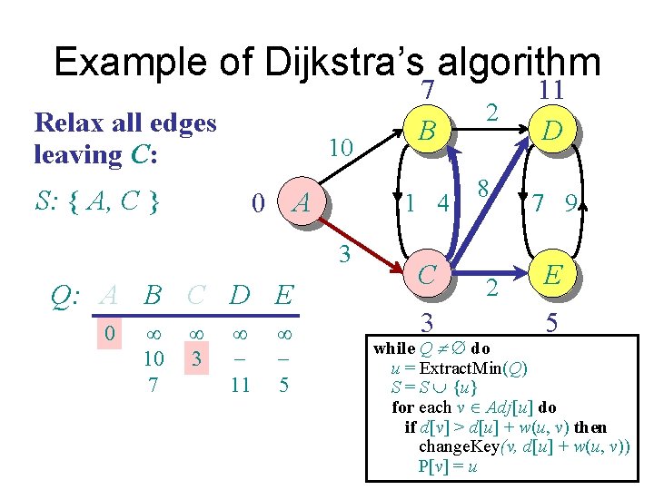
Example of Dijkstra’s algorithm Relax all edges leaving C: 10 S: { A, C } 0 A 1 4 3 Q: A B C D E 0 ¥ 10 7 ¥ 3 ¥ 11 ¥ 5 7 B C 3 2 8 2 11 D 7 9 E 5 while Q ¹ do u = Extract. Min(Q) S = S È {u} for each v Î Adj[u] do if d[v] > d[u] + w(u, v) then change. Key(v, d[u] + w(u, v)) P[v] = u

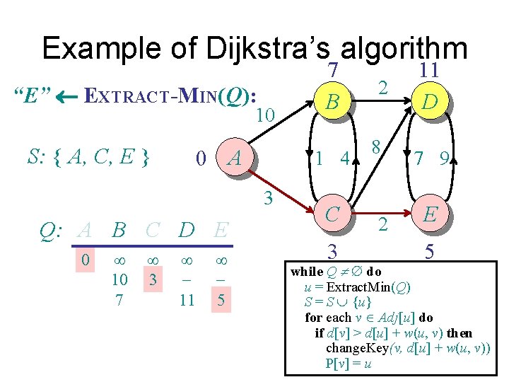
Example of Dijkstra’s algorithm “E” EXTRACT-MIN(Q): 10 S: { A, C, E } 0 A 1 4 3 Q: A B C D E 0 ¥ 10 7 ¥ 3 ¥ 11 ¥ 5 7 B C 3 2 8 2 11 D 7 9 E 5 while Q ¹ do u = Extract. Min(Q) S = S È {u} for each v Î Adj[u] do if d[v] > d[u] + w(u, v) then change. Key(v, d[u] + w(u, v)) P[v] = u

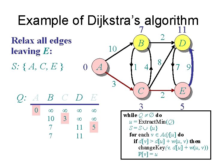
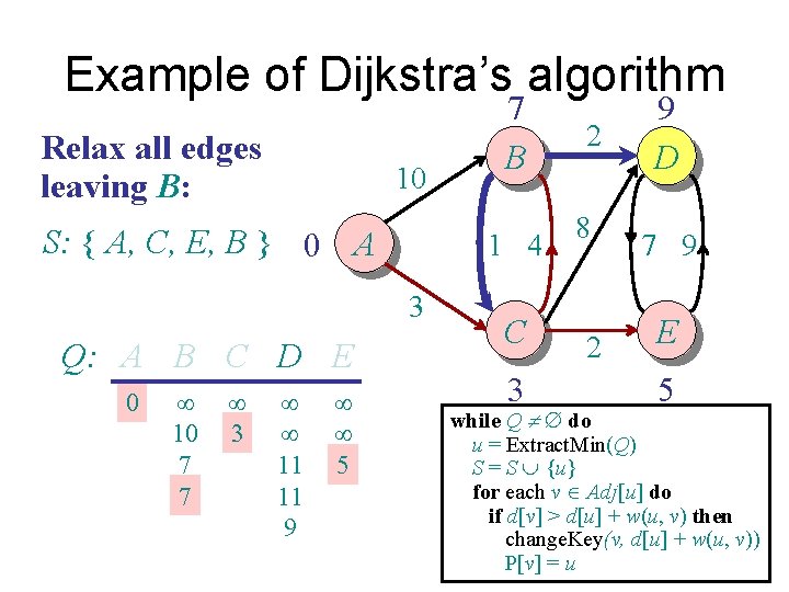
Example of Dijkstra’s algorithm Relax all edges leaving E: 10 S: { A, C, E } 0 A 1 4 3 Q: A B C D E 0 ¥ 10 7 7 ¥ 3 ¥ ¥ 11 11 ¥ ¥ 5 7 B C 3 2 8 2 11 D 7 9 E 5 while Q ¹ do u = Extract. Min(Q) S = S È {u} for each v Î Adj[u] do if d[v] > d[u] + w(u, v) then change. Key(v, d[u] + w(u, v)) P[v] = u

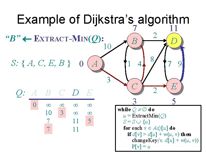
Example of Dijkstra’s algorithm “B” EXTRACT-MIN(Q): 10 S: { A, C, E, B } 0 A 1 4 3 Q: A B C D E 0 ¥ 10 7 7 ¥ 3 ¥ ¥ 11 11 ¥ ¥ 5 7 B C 3 2 8 2 11 D 7 9 E 5 while Q ¹ do u = Extract. Min(Q) S = S È {u} for each v Î Adj[u] do if d[v] > d[u] + w(u, v) then change. Key(v, d[u] + w(u, v)) P[v] = u

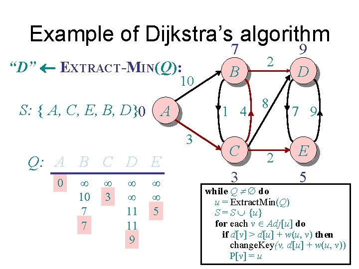
Example of Dijkstra’s algorithm Relax all edges leaving B: 10 S: { A, C, E, B } 0 A 1 4 3 Q: A B C D E 0 ¥ 10 7 7 ¥ 3 ¥ ¥ 11 11 9 ¥ ¥ 5 7 B C 3 2 8 2 9 D 7 9 E 5 while Q ¹ do u = Extract. Min(Q) S = S È {u} for each v Î Adj[u] do if d[v] > d[u] + w(u, v) then change. Key(v, d[u] + w(u, v)) P[v] = u

Example of Dijkstra’s algorithm “D” EXTRACT-MIN(Q): 10 S: { A, C, E, B, D}0 A 1 4 3 Q: A B C D E 0 ¥ 10 7 7 ¥ 3 ¥ ¥ 11 11 9 ¥ ¥ 5 7 B C 3 2 8 2 9 D 7 9 E 5 while Q ¹ do u = Extract. Min(Q) S = S È {u} for each v Î Adj[u] do if d[v] > d[u] + w(u, v) then change. Key(v, d[u] + w(u, v)) P[v] = u

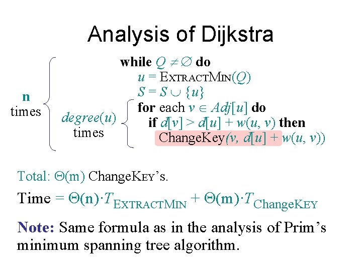
Analysis of Dijkstra n times while Q ¹ do u = EXTRACTMIN(Q) S = S È {u} for each v Î Adj[u] do degree(u) if d[v] > d[u] + w(u, v) then times Change. Key(v, d[u] + w(u, v)) Total: Q(m) Change. KEY’s. Time = Q(n)·TEXTRACTMIN + Q(m)·TChange. KEY Note: Same formula as in the analysis of Prim’s minimum spanning tree algorithm.

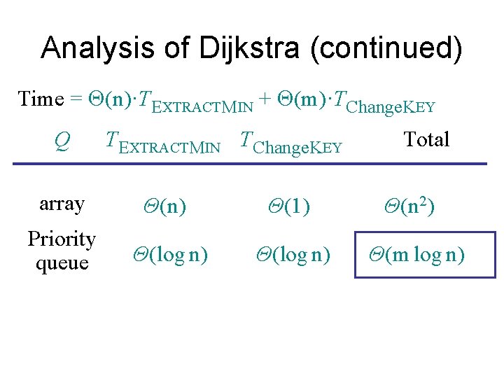
Analysis of Dijkstra (continued) Time = Q(n)·TEXTRACTMIN + Q(m)·TChange. KEY Q TEXTRACTMIN TChange. KEY array Θ(n) Θ(1) Priority queue Θ(log n) Total Θ(n 2) Θ(m log n)

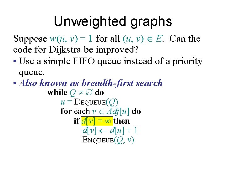
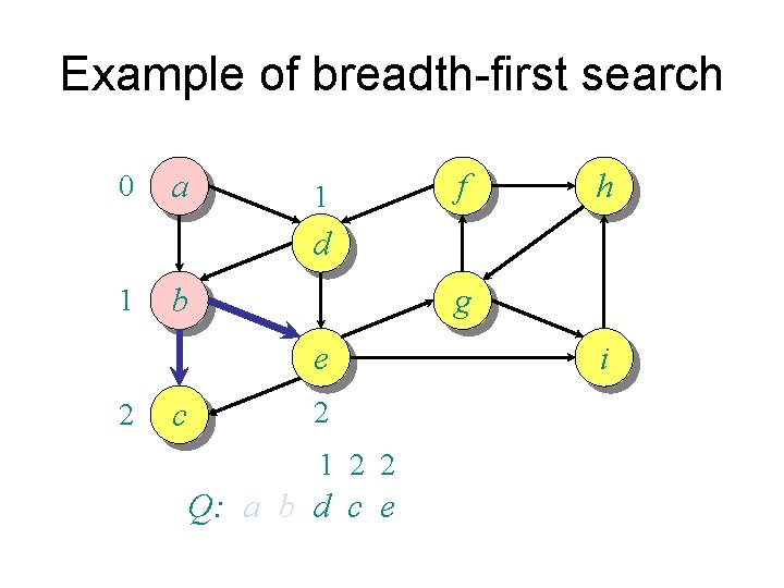
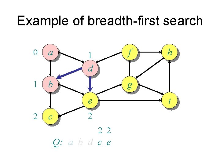
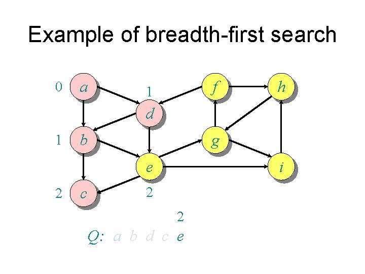
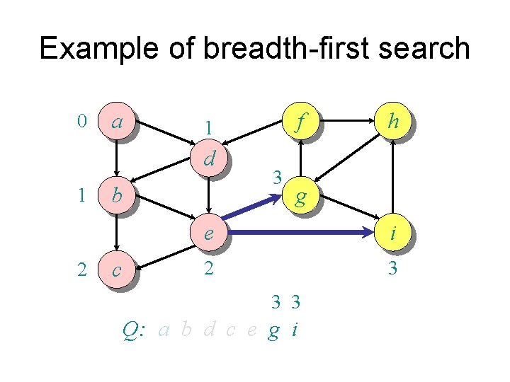
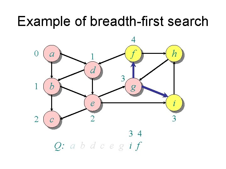
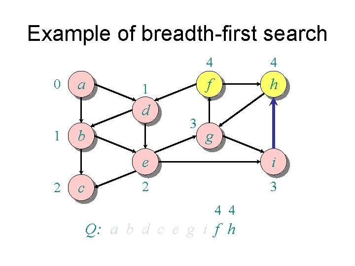
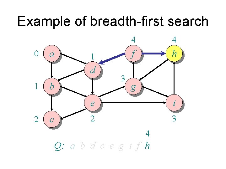
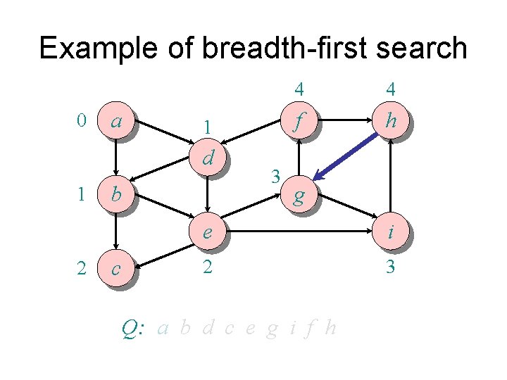
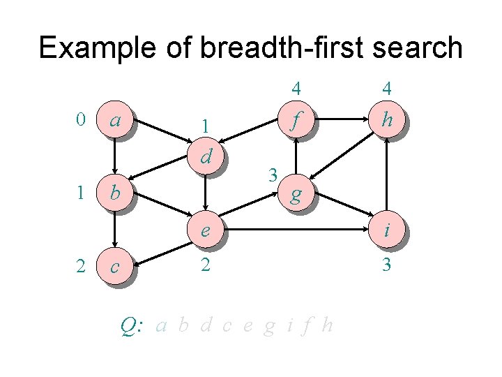
Unweighted graphs Suppose w(u, v) = 1 for all (u, v) Î E. Can the code for Dijkstra be improved? • Use a simple FIFO queue instead of a priority queue. • Also known as breadth-first search while Q ¹ do u = DEQUEUE(Q) for each v Î Adj[u] do if d[v] = ¥ then d[v] d[u] + 1 ENQUEUE(Q, v)

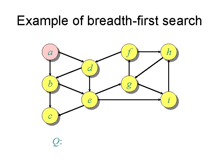
Example of breadth-first search a f h d b g e c Q: i

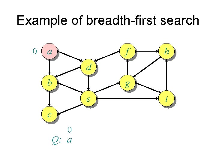
Example of breadth-first search 0 a f h d b g e c 0 Q: a i

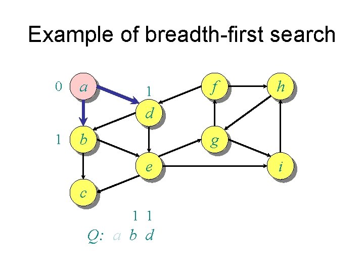
Example of breadth-first search 0 a 1 f h d 1 b g e c 1 1 Q: a b d i

Example of breadth-first search 0 a 1 f h d 1 b g e 2 c 2 1 2 2 Q: a b d c e i

Example of breadth-first search 0 a f 1 h d 1 b g e 2 c i 2 2 2 Q: a b d c e

Example of breadth-first search 0 a f 1 h d 1 b g e 2 c i 2 2 Q: a b d c e

Example of breadth-first search 0 a d 1 2 b c f 1 3 h g e i 2 3 3 3 Q: a b d c e g i

Example of breadth-first search 4 0 a d 1 2 b c f 1 3 h g e i 2 3 3 4 Q: a b d c e g i f

Example of breadth-first search 0 a 1 d 1 2 b c 3 4 4 f h g e i 2 3 4 4 Q: a b d c e g i f h

Example of breadth-first search 0 a 1 d 1 2 b c 3 4 4 f h g e i 2 3 4 Q: a b d c e g i f h

Example of breadth-first search 0 a 1 d 1 2 b c 3 4 4 f h g e i 2 3 Q: a b d c e g i f h

Example of breadth-first search 0 a 1 d 1 2 b c 3 4 4 f h g e i 2 3 Q: a b d c e g i f h

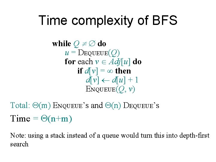
Time complexity of BFS while Q ¹ do u = DEQUEUE(Q) for each v Î Adj[u] do if d[v] = ¥ then d[v] d[u] + 1 ENQUEUE(Q, v) Total: Q(m) ENQUEUE’s and Q(n) DEQUEUE’s Time = Q(n+m) Note: using a stack instead of a queue would turn this into depth-first search