Introduction to the Design and Analysis of Algorithms

Introduction to the Design and Analysis of Algorithms El. Sayed Badr Benha University September 20, 2016

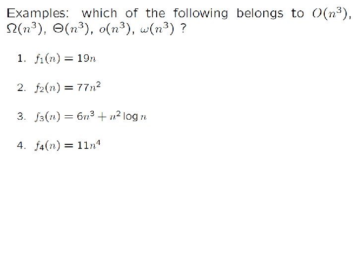
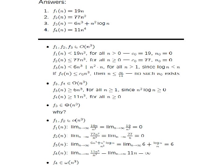
Problem: 2

Problem: 3

Big-oh

Big-omega

Big-theta

Establishing order of growth using the definition Definition: f(n) is in O(g(n)), denoted f(n) O(g(n)), if order of growth of f(n) ≤ order of growth of g(n) (within constant multiple), i. e. , there exist a positive constant c and non-negative integer n 0 such that f(n) ≤ c g(n) for every n ≥ n 0 0 -notation The bound is asymptotically Examples: tight 2 • 10 n is in O(n ) But the bound is not. But we can write little o-notation • 5 n+20 is in O(n) Example :

-notation • Formal definition – A function t(n) is said to be in (g(n)), denoted t(n) (g(n)), if t(n) is bounded below by some constant multiple of g(n) for all large n, i. e. , if there exist some positive constant c and some nonnegative integer n 0 such that t(n) cg(n) for all n n 0 • Examples: – 10 n 2 (n 2) – 0. 3 n 2 - 2 n (n 2) – 0. 1 n 3 (n 2) Example :

-notation • Formal definition – A function t(n) is said to be in (g(n)), denoted t(n) (g(n)), if t(n) is bounded both above and below by some positive constant multiples of g(n) for all large n, i. e. , if there exist some positive constant c 1 and c 2 and some nonnegative integer n 0 such that c 2 g(n) t(n) c 1 g(n) for all n n 0 • Examples: – 10 n 2 (n 2) – 0. 3 n 2 - 2 n (n 2) – (1/2)n(n+1) (n 2)

>= (g(n)), functions that grow at least as fast as g(n) = (g(n)), functions that grow at the same rate as g(n) <= O(g(n)), functions that grow no faster than g(n)

Logarithm Review

Logarithm Review

Useful summation formulas and rules l I n 1 = 1+1+…+1 = n - l + 1 In particular, l I n 1 = n - 1 + 1 = n (n) 1 i n i = 1+2+…+n = n(n+1)/2 n 2/2 (n 2) 1 i n i 2 = 12+22+…+n 2 = n(n+1)(2 n+1)/6 n 3/3 (n 3) 0 i n ai = 1 + a +…+ an = (an+1 - 1)/(a - 1) for any a 1 In particular, 0 i n 2 i = 20 + 21 +…+ 2 n = 2 n+1 - 1 (2 n ) (ai ± bi ) = ai ± bi m+1 i uai cai = c ai l i uai = l i mai +

Example 1: Maximum element

Example 2: Element uniqueness problem

Example 3: Matrix multiplication

Example 4: Gaussian elimination Algorithm Gaussian. Elimination(A[0. . n-1, 0. . n]) //Implements Gaussian elimination on an n- by-(n + 1) matrix A for i 0 to n - 2 do for j i + 1 to n - 1 do for k i to n do A[j, k] - A[i, k] A[j, i] / A[i, i]

Plan for Analysis of Recursive Algorithms • Decide on a parameter indicating an input’s size. • Identify the algorithm’s basic operation. • Check whether the number of times the basic op. is executed may vary on different inputs of the same size. (If it may, the worst, average, and best cases must be investigated separately. ) • Set up a recurrence relation with an appropriate initial condition expressing the number of times the basic op. is executed. • Solve the recurrence (or, at the very least, establish its solution’s order of growth) by backward substitutions or another method.

Example 1: Recursive evaluation of n! Definition: n ! = 1 2 … (n-1) n for n ≥ 1 and 0! = 1 Recursive definition of n!: F(n) = F(n-1) n for n ≥ 1 and F(0) = 1 n Size: Basic operation: Recurrence relation: multiplication M(n) = M(n-1) + 1 M(0) = 0

Solving the recurrence for M(n) = M(n-1) + 1, M(0) = 0 M(n) = M(n-1) + 1 = (M(n-2) + 1 = M(n-2) + 2 = (M(n-3) + 1) + 2 = M(n-3) + 3 … = M(n-i) + i = M(0) + n =n The method is called backward substitution.

Smoothness Rule • Let f(n) be a nonnegative function defined on the set of natural numbers. f(n) is call smooth if it is eventually nondecreasing and f(2 n) ∈ Θ (f(n)) – Functions that do not grow too fast, including logn, n, nlogn, and n where >=0 are smooth. • Smoothness rule Let T(n) be an eventually nondecreasing function and f(n) be a smooth function. If T(n) ∈ Θ (f(n)) for values of n that are powers of b, where b>=2, then T(n) ∈ Θ (f(n)) for any n.

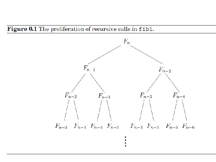
Fibonacci numbers The Fibonacci numbers: 0, 1, 1, 2, 3, 5, 8, 13, 21, … The Fibonacci recurrence: F(n) = F(n-1) + F(n-2) F(0) = 0 F(1) = 1 In fact, the Fibonacci numbers grow almost as fast as the powers of 2: for example, F 30 is over a million, and F 100 is already 21 digits long! In general, Fn ≈ 20: 694 n But what is the precise value of F 100, or of F 200 ? Fibonacci himself would surely have wanted to know such things.

Fibonacci numbers function fib 1(n) if n = 0: return 0 if n = 1: return 1 return fib 1(n - 1) + fib 1(n - 2) we immediately see that At this time, the fastest computer in the world is the NEC Earth Simulator, which clocks 40 trillion steps per second. Even on this machine, fib 1(200) would take at least 292 seconds.

Fibonacci numbers function fib 2(n) if n = 0 return 0 create an array f[0 …n] f[0] = 0, f[1] = 1 for i = 2 …n: f[i] = f[i - 1] + f[i - 2] return f[n] General 2 nd order linear homogeneous recurrence with constant coefficients: a. X(n) + b. X(n-1) + c. X(n-2) = 0

Solving a. X(n) + b. X(n-1) + c. X(n-2) = 0 • Set up the characteristic equation (quadratic) ar 2 + br + c = 0 • Solve to obtain roots r 1 and r 2 • General solution to the recurrence if r 1 and r 2 are two distinct real roots: X(n) = αr 1 n + βr 2 n if r 1 = r 2 = r are two equal real roots: X(n) = αrn + βnr n • Particular solution can be found by using initial conditions

Application to the Fibonacci numbers F(n) = F(n-1) + F(n-2) or F(n) - F(n-1) - F(n-2) = 0 Characteristic equation: Roots of the characteristic equation: General solution to the recurrence: Particular solution for F(0) =0, F(1)=1:

Computing Fibonacci numbers 1. Definition-based recursive algorithm 2. Nonrecursive definition-based algorithm 3. Explicit formula algorithm 4. Logarithmic algorithm based on formula: F(n-1) F(n) F(n+1) = 0 1 1 n 1 for n ≥ 1, assuming an efficient way of computing matrix powers.

Important Recurrence Types • • Decrease-by-one recurrences – A decrease-by-one algorithm solves a problem by exploiting a relationship between a given instance of size n and a smaller size n – 1. – Example: n! – The recurrence equation for investigating the time efficiency of such algorithms typically has the form T(n) = T(n-1) + f(n) Decrease-by-a-constant-factor recurrences – A decrease-by-a-constant-factor algorithm solves a problem by dividing its given instance of size n into several smaller instances of size n/b, solving each of them recursively, and then, if necessary, combining the solutions to the smaller instances into a solution to the given instance. – Example: binary search. – The recurrence equation for investigating the time efficiency of such algorithms typically has the form T(n) = a. T(n/b) + f (n)

Decrease-by-one Recurrences • One (constant) operation reduces problem size by one. T(n) = T(n-1) + c T(1) = d Solution: T(n) = (n-1)c + d • linear A pass through input reduces problem size by one. T(n) = T(n-1) + c n T(1) = d Solution: T(n) = [n(n+1)/2 – 1] c + d quadratic

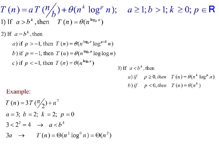
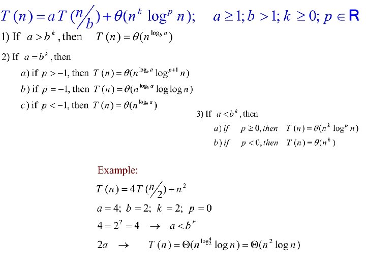
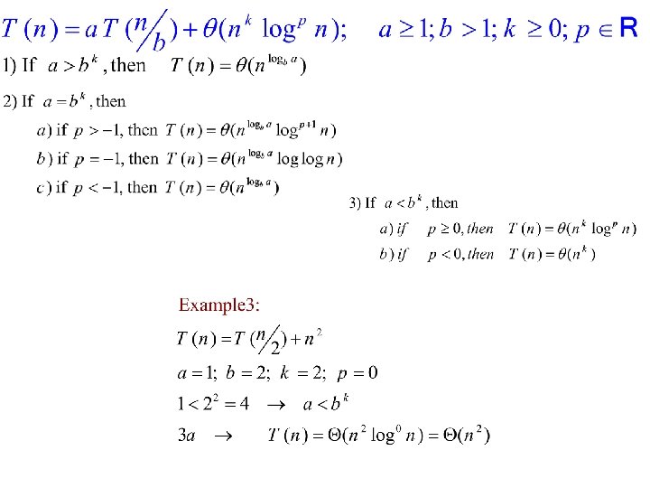
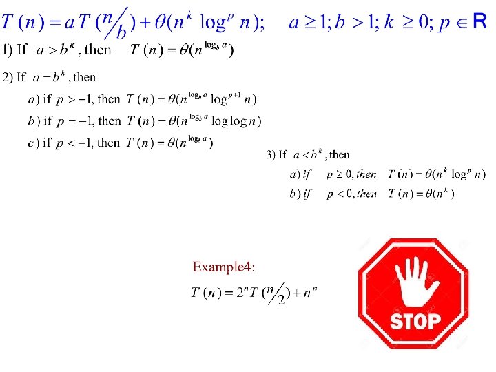
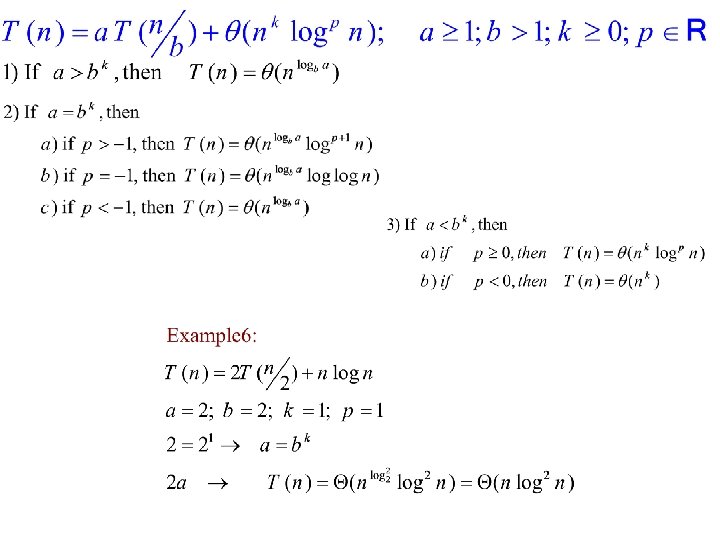
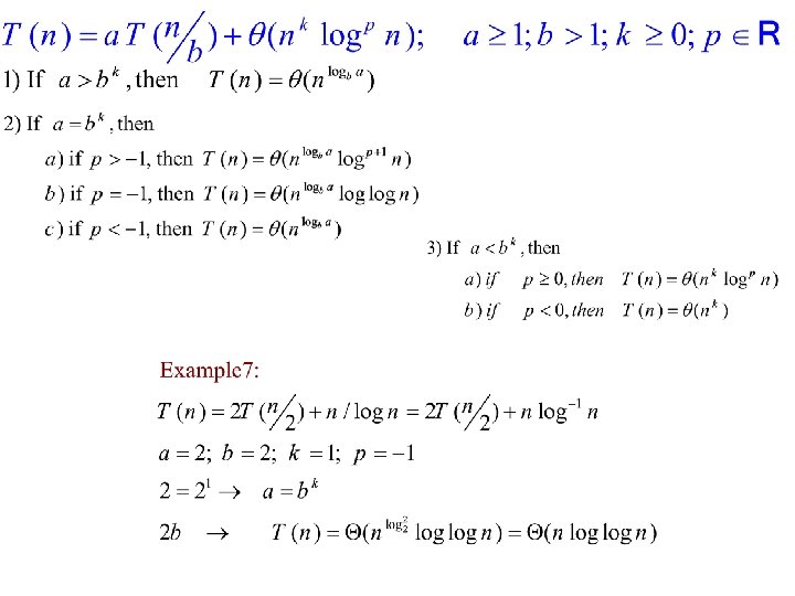
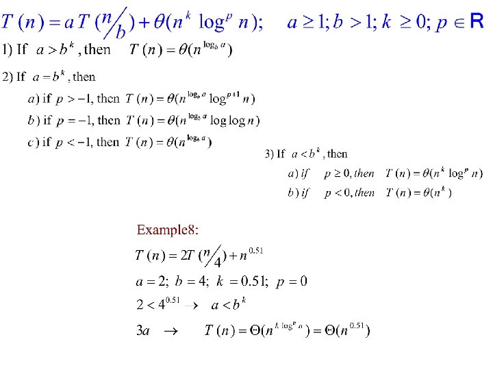
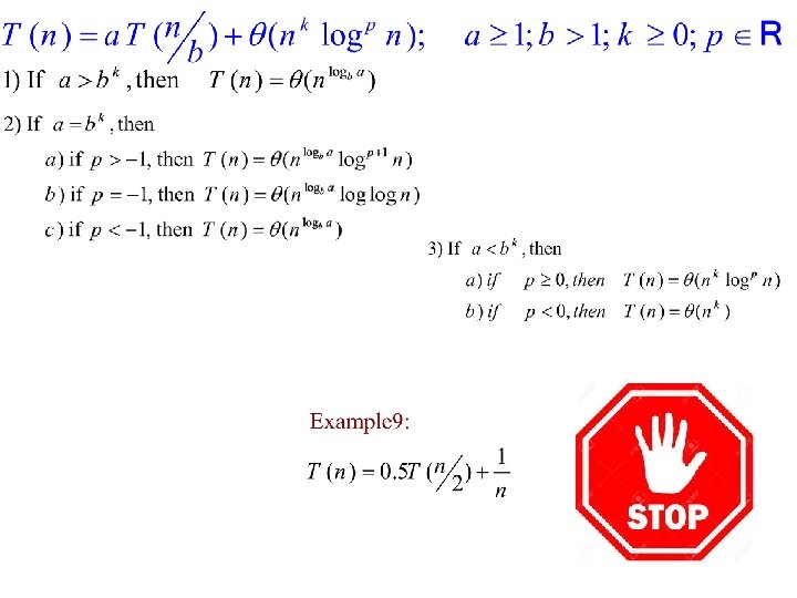
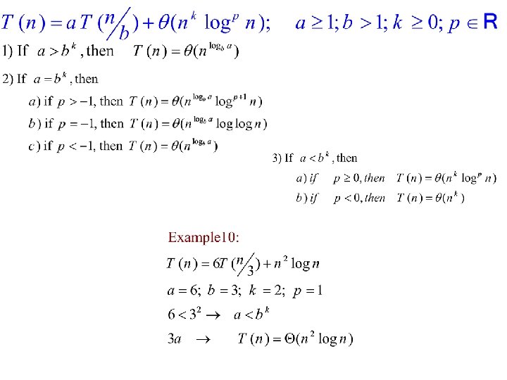
Master Theorem