CS 3343 Analysis of Algorithms Linear time sorting

CS 3343: Analysis of Algorithms Linear time sorting algorithms

More about sorting • How many sorting algorithms do you know? • What are their time complexity? • What’s common about them? • Can we do better than Θ(n log n)? • Yes and no

Outline • More about sorting – Theoretical lower-bound – Linear-time sorting algorithms – Stability of sorting

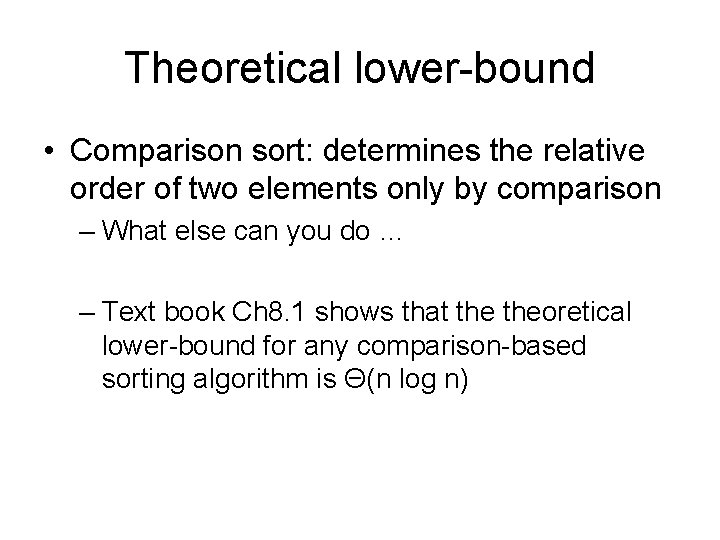
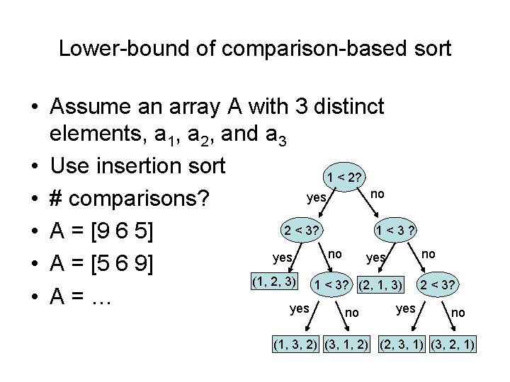
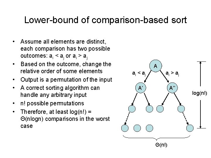
Theoretical lower-bound • Comparison sort: determines the relative order of two elements only by comparison – What else can you do … – Text book Ch 8. 1 shows that theoretical lower-bound for any comparison-based sorting algorithm is Θ(n log n)

Lower-bound of comparison-based sort • Assume an array A with 3 distinct elements, a 1, a 2, and a 3 • Use insertion sort 1 < 2? no yes • # comparisons? 2 < 3? 1<3? • A = [9 6 5] no no yes • A = [5 6 9] (1, 2, 3) 1 < 3? (2, 1, 3) 2 < 3? • A=… yes no no (1, 3, 2) (3, 1, 2) (2, 3, 1) (3, 2, 1)

Lower-bound of comparison-based sort • Assume all elements are distinct, each comparison has two possible outcomes: ai < aj or ai > aj • Based on the outcome, change the relative order of some elements • Output is a permutation of the input • A correct sorting algorithm can handle any arbitrary input • n! possible permutations • Therefore, at least log(n!) = Θ(nlogn) comparisons in the worst case A ai < a j ai > a j A’ A’’ Θ(n!) log(n!)

Sorting in linear time • Is there a problem with theory? • No. We are going to sort without doing comparison • How is that possible? • Key: knowledge about the data – Example: Almost sorted? All distinct? Many identical ones? Uniformly distributed? – The more you know about your data, the more likely you can have a better algorithm

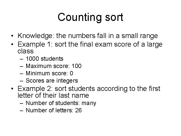
Counting sort • Knowledge: the numbers fall in a small range • Example 1: sort the final exam score of a large class – – 1000 students Maximum score: 100 Minimum score: 0 Scores are integers • Example 2: sort students according to the first letter of their last name – Number of students: many – Number of letters: 26

Counting sort • Input: A[1. . n], where A[ j]Î{1, 2, …, k}. • Output: B[1. . n], sorted. • Auxiliary storage: C[1. . k]. • Not an in-place sorting algorithm • Requires (n+k) additional storage besides the original array

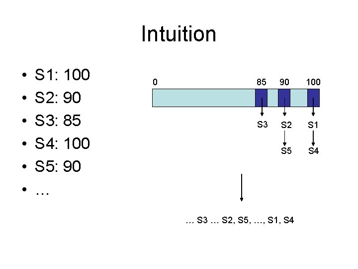
Intuition • • • S 1: 100 S 2: 90 S 3: 85 S 4: 100 S 5: 90 … 0 85 90 100 S 3 S 2 S 1 S 5 S 4 … S 3 … S 2, S 5, …, S 1, S 4

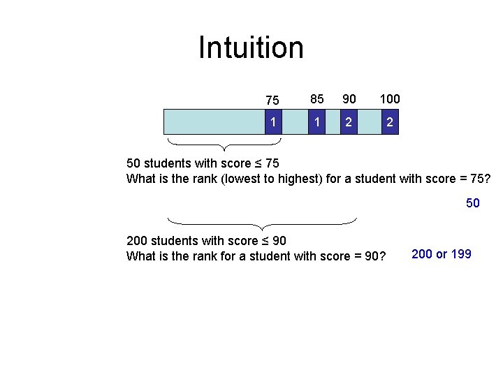
Intuition 75 85 90 100 1 1 2 2 50 students with score ≤ 75 What is the rank (lowest to highest) for a student with score = 75? 50 200 students with score ≤ 90 What is the rank for a student with score = 90? 200 or 199

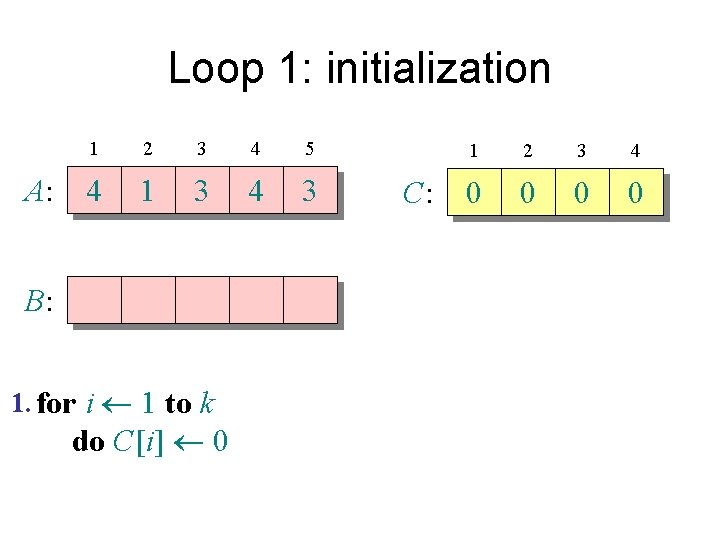
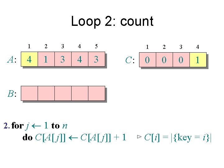
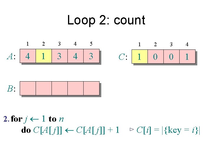
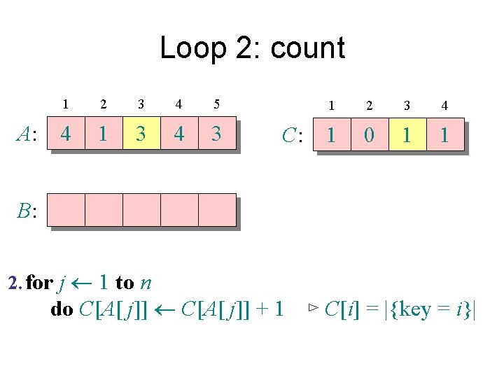
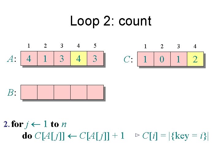
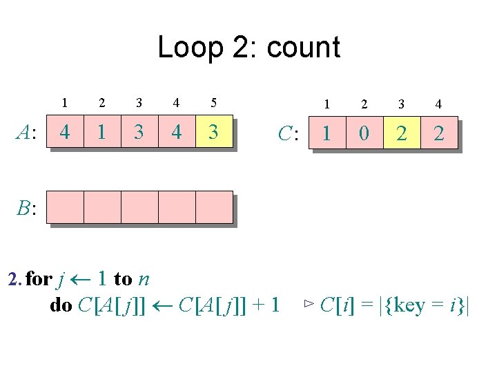
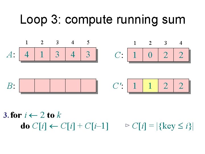
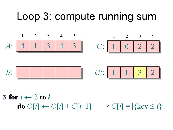
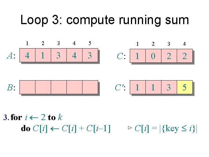
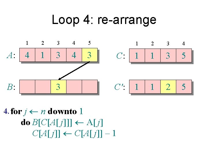
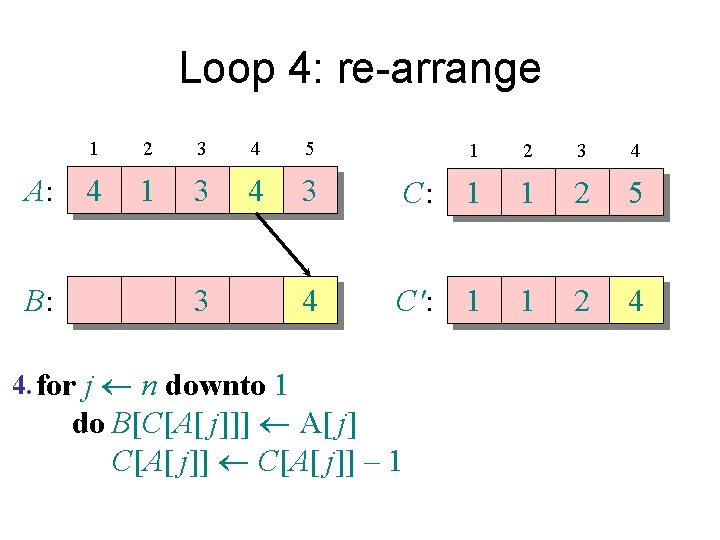
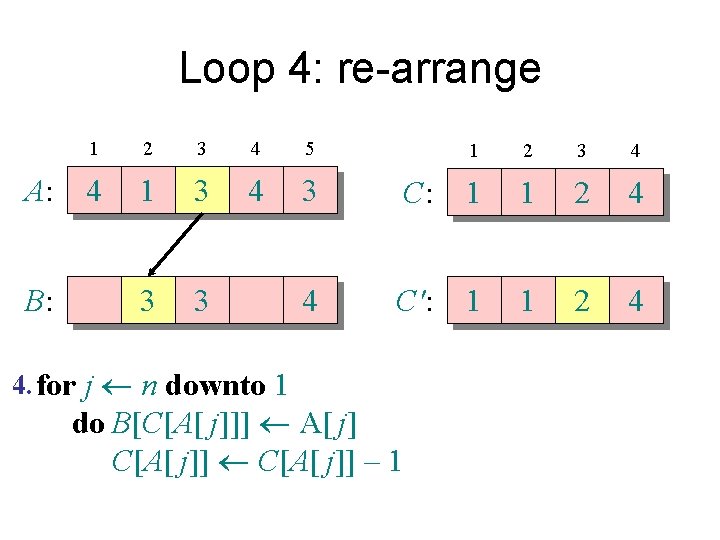
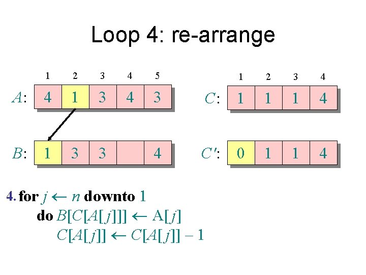
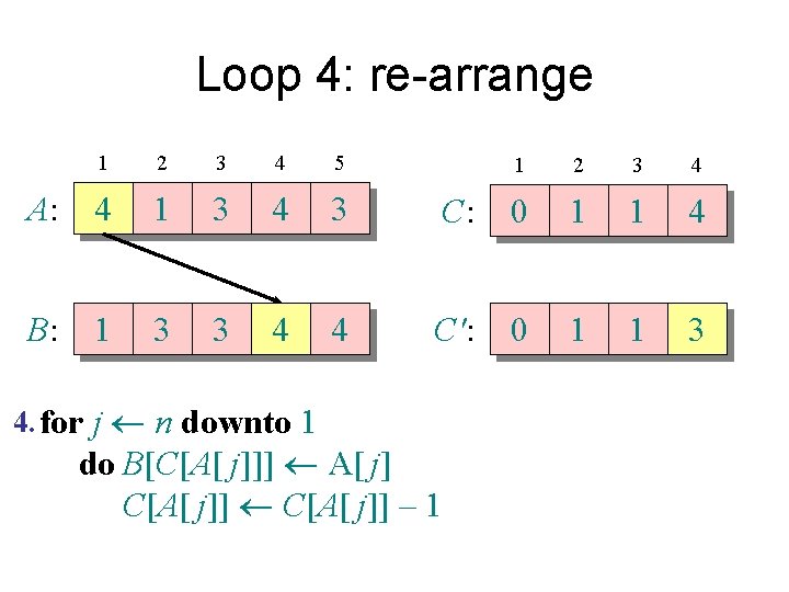
Counting sort 1. for i 1 to k Initialize do C[i] 0 Count 2. for j 1 to n do C[A[ j]] + 1 ⊳ C[i] = |{key = i}| Compute running sum 3. for i 2 to k do C[i] + C[i– 1] ⊳ C[i] = |{key £ i}| 4. for j n downto 1 Re-arrange do B[C[A[ j]]] A[ j] C[A[ j]] – 1

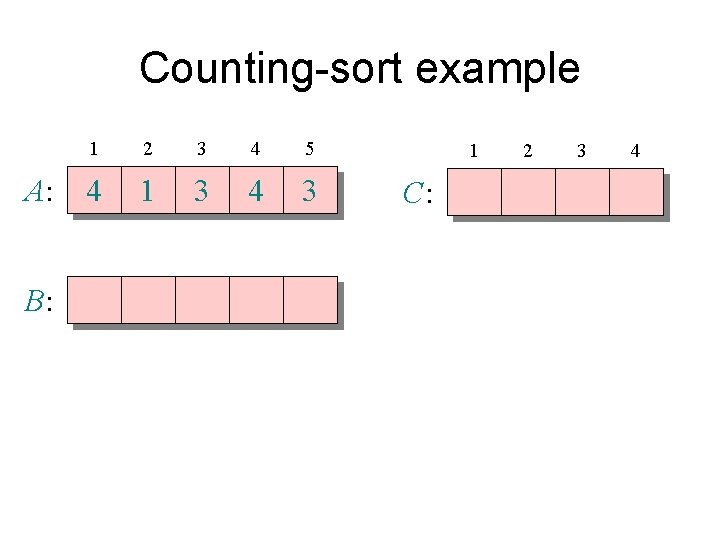
Counting-sort example A: B: 1 2 3 4 5 4 1 3 4 3 1 C: 2 3 4

Loop 1: initialization A: 1 2 3 4 5 4 1 3 4 3 B: 1. for i 1 to k do C[i] 0 C: 1 2 3 4 0 0

Loop 2: count A: 1 2 3 4 5 4 1 3 4 3 C: 1 2 3 4 0 0 0 1 B: 2. for j 1 to n do C[A[ j]] + 1 ⊳ C[i] = |{key = i}|

Loop 2: count A: 1 2 3 4 5 4 1 3 4 3 C: 1 2 3 4 1 0 0 1 B: 2. for j 1 to n do C[A[ j]] + 1 ⊳ C[i] = |{key = i}|

Loop 2: count A: 1 2 3 4 5 4 1 3 4 3 C: 1 2 3 4 1 0 1 1 B: 2. for j 1 to n do C[A[ j]] + 1 ⊳ C[i] = |{key = i}|

Loop 2: count A: 1 2 3 4 5 4 1 3 4 3 C: 1 2 3 4 1 0 1 2 B: 2. for j 1 to n do C[A[ j]] + 1 ⊳ C[i] = |{key = i}|

Loop 2: count A: 1 2 3 4 5 4 1 3 4 3 C: 1 2 3 4 1 0 2 2 B: 2. for j 1 to n do C[A[ j]] + 1 ⊳ C[i] = |{key = i}|

Loop 3: compute running sum A: 1 2 3 4 5 4 1 3 4 3 B: 3. for i 2 to k do C[i] + C[i– 1] 1 2 3 4 C: 1 0 2 2 C': 1 1 2 2 ⊳ C[i] = |{key £ i}|

Loop 3: compute running sum A: 1 2 3 4 5 4 1 3 4 3 B: 3. for i 2 to k do C[i] + C[i– 1] 1 2 3 4 C: 1 0 2 2 C': 1 1 3 2 ⊳ C[i] = |{key £ i}|

Loop 3: compute running sum A: 1 2 3 4 5 4 1 3 4 3 B: 3. for i 2 to k do C[i] + C[i– 1] 1 2 3 4 C: 1 0 2 2 C': 1 1 3 5 ⊳ C[i] = |{key £ i}|

Loop 4: re-arrange A: B: 1 2 3 4 5 4 1 3 4 3 3 4. for j n downto 1 1 2 3 4 C: 1 1 3 5 C': 1 1 3 5 do B[C[A[ j]]] A[ j] C[A[ j]] – 1

Loop 4: re-arrange A: B: 1 2 3 4 5 4 1 3 4 3 3 4. for j n downto 1 1 2 3 4 C: 1 1 3 5 C': 1 1 2 5 do B[C[A[ j]]] A[ j] C[A[ j]] – 1

Loop 4: re-arrange A: B: 1 2 3 4 5 4 1 3 4 3 4. for j n downto 1 1 2 3 4 C: 1 1 2 5 C': 1 1 2 5 do B[C[A[ j]]] A[ j] C[A[ j]] – 1

Loop 4: re-arrange A: B: 1 2 3 4 5 4 1 3 4 3 4. for j n downto 1 1 2 3 4 C: 1 1 2 5 C': 1 1 2 4 do B[C[A[ j]]] A[ j] C[A[ j]] – 1

Loop 4: re-arrange A: B: 1 2 3 4 5 4 1 3 4 3 3 3 4 4. for j n downto 1 1 2 3 4 C: 1 1 2 4 C': 1 1 2 4 do B[C[A[ j]]] A[ j] C[A[ j]] – 1

Loop 4: re-arrange A: B: 1 2 3 4 5 4 1 3 4 3 3 3 4 4. for j n downto 1 1 2 3 4 C: 1 1 2 4 C': 1 1 1 4 do B[C[A[ j]]] A[ j] C[A[ j]] – 1

Loop 4: re-arrange 1 2 3 4 5 A: 4 1 3 4 3 B: 1 3 3 4 4. for j n downto 1 1 2 3 4 C: 1 1 1 4 C': 1 1 1 4 do B[C[A[ j]]] A[ j] C[A[ j]] – 1

Loop 4: re-arrange 1 2 3 4 5 A: 4 1 3 4 3 B: 1 3 3 4 4. for j n downto 1 1 2 3 4 C: 1 1 1 4 C': 0 1 1 4 do B[C[A[ j]]] A[ j] C[A[ j]] – 1

Loop 4: re-arrange 1 2 3 4 5 A: 4 1 3 4 3 B: 1 3 3 4 4 4. for j n downto 1 1 2 3 4 C: 0 1 1 4 C': 0 1 1 4 do B[C[A[ j]]] A[ j] C[A[ j]] – 1

Loop 4: re-arrange 1 2 3 4 5 A: 4 1 3 4 3 B: 1 3 3 4 4 4. for j n downto 1 1 2 3 4 C: 0 1 1 4 C': 0 1 1 3 do B[C[A[ j]]] A[ j] C[A[ j]] – 1

Analysis (k) (n) (n + k) 1. for i 1 to k do C[i] 0 2. for j 1 to n do C[A[ j]] + 1 3. for i 2 to k do C[i] + C[i– 1] 4. for j n downto 1 do B[C[A[ j]]] A[ j] C[A[ j]] – 1

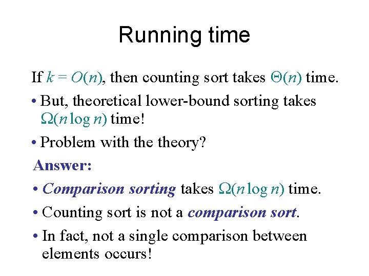
Running time If k = O(n), then counting sort takes (n) time. • But, theoretical lower-bound sorting takes W(n log n) time! • Problem with theory? Answer: • Comparison sorting takes W(n log n) time. • Counting sort is not a comparison sort. • In fact, not a single comparison between elements occurs!

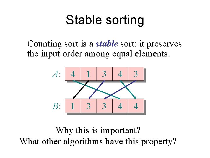
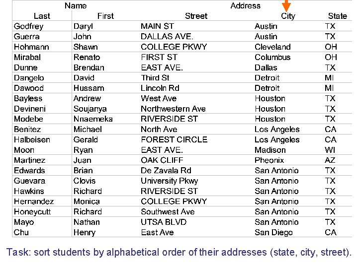
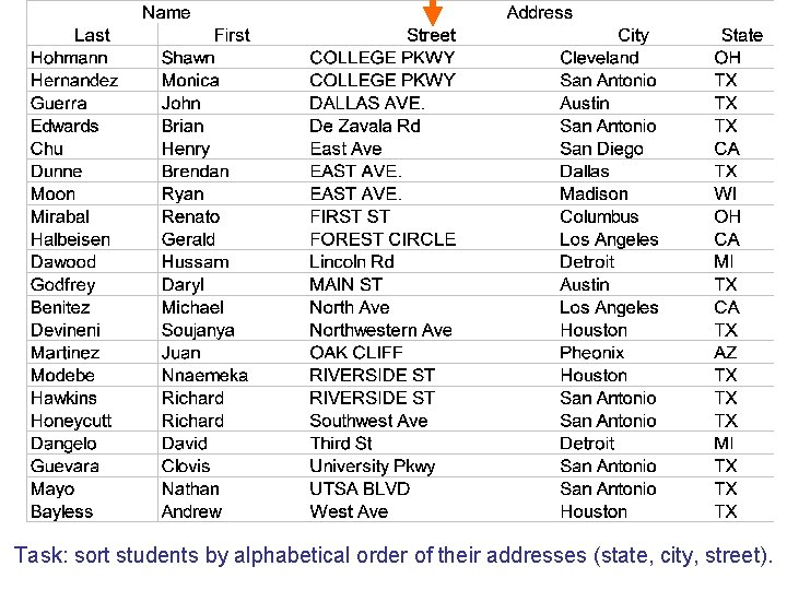
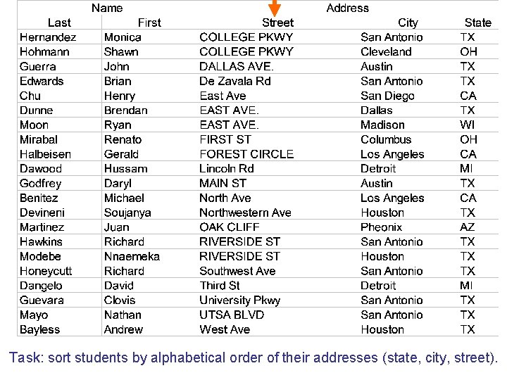
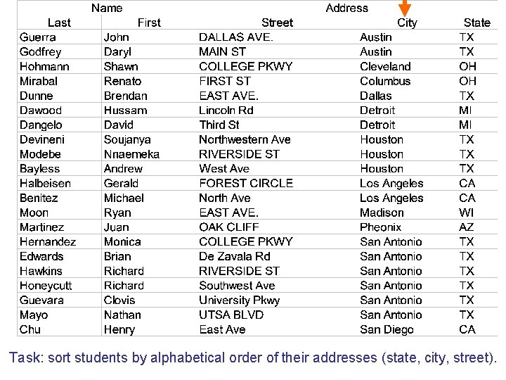
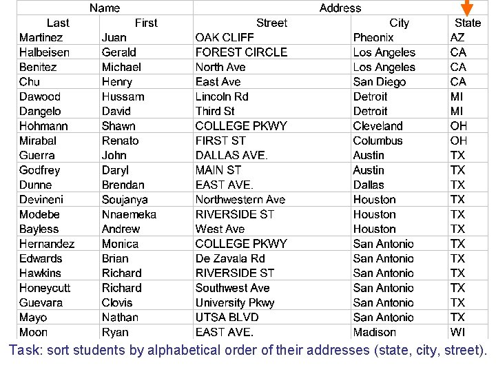
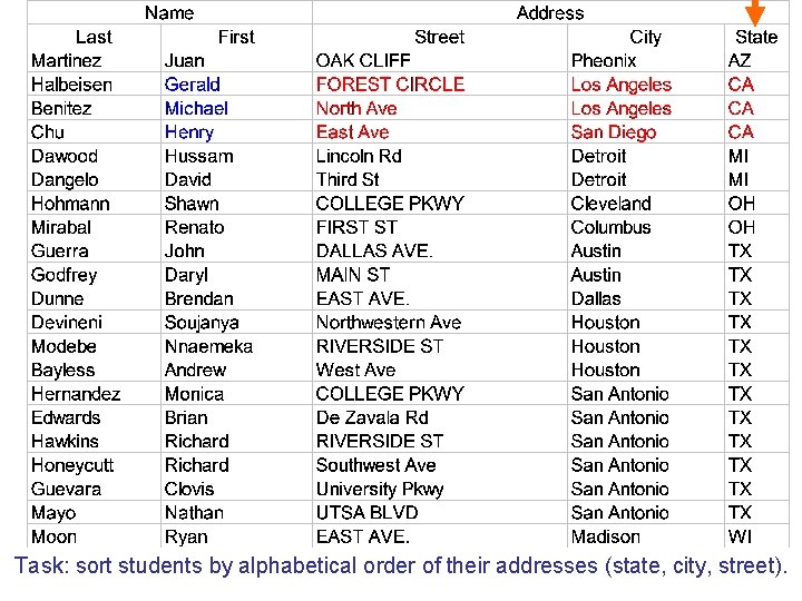
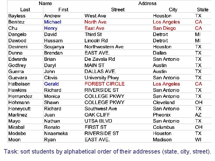
Stable sorting Counting sort is a stable sort: it preserves the input order among equal elements. A: 4 1 3 4 3 B: 1 3 3 4 4 Why this is important? What other algorithms have this property?

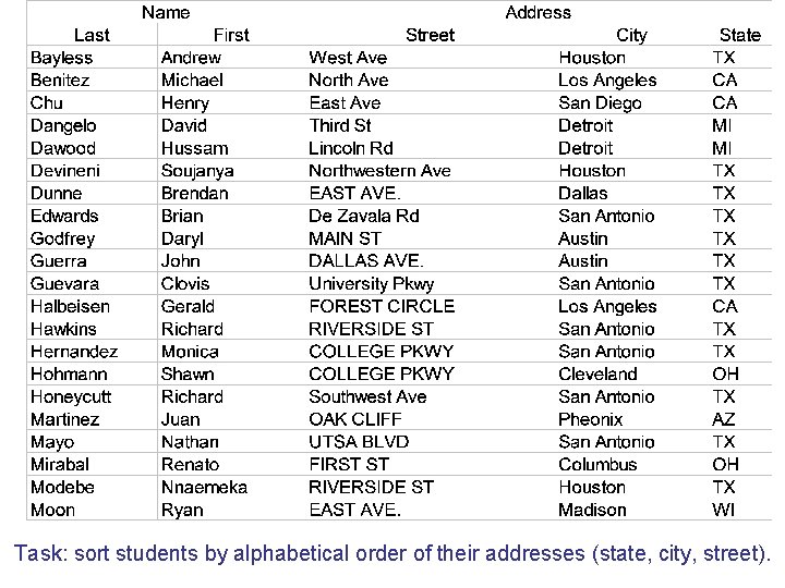
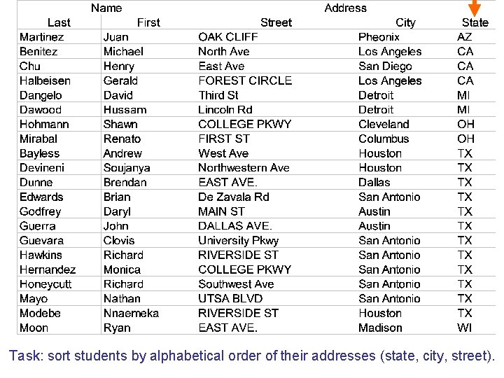
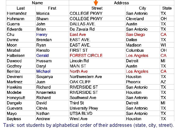
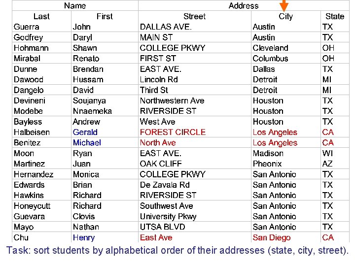
Task: sort students by alphabetical order of their addresses (state, city, street).

Task: sort students by alphabetical order of their addresses (state, city, street).

Task: sort students by alphabetical order of their addresses (state, city, street).

Task: sort students by alphabetical order of their addresses (state, city, street).

Task: sort students by alphabetical order of their addresses (state, city, street).

Task: sort students by alphabetical order of their addresses (state, city, street).

Task: sort students by alphabetical order of their addresses (state, city, street).

Task: sort students by alphabetical order of their addresses (state, city, street).

Task: sort students by alphabetical order of their addresses (state, city, street).

Task: sort students by alphabetical order of their addresses (state, city, street).

Task: sort students by alphabetical order of their addresses (state, city, street).

Task: sort students by alphabetical order of their addresses (state, city, street).

Task: sort students by alphabetical order of their addresses (state, city, street).

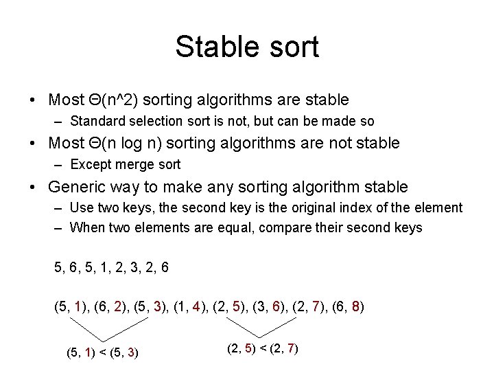
Stable sort • Most Θ(n^2) sorting algorithms are stable – Standard selection sort is not, but can be made so • Most Θ(n log n) sorting algorithms are not stable – Except merge sort • Generic way to make any sorting algorithm stable – Use two keys, the second key is the original index of the element – When two elements are equal, compare their second keys 5, 6, 5, 1, 2, 3, 2, 6 (5, 1), (6, 2), (5, 3), (1, 4), (2, 5), (3, 6), (2, 7), (6, 8) (5, 1) < (5, 3) (2, 5) < (2, 7)

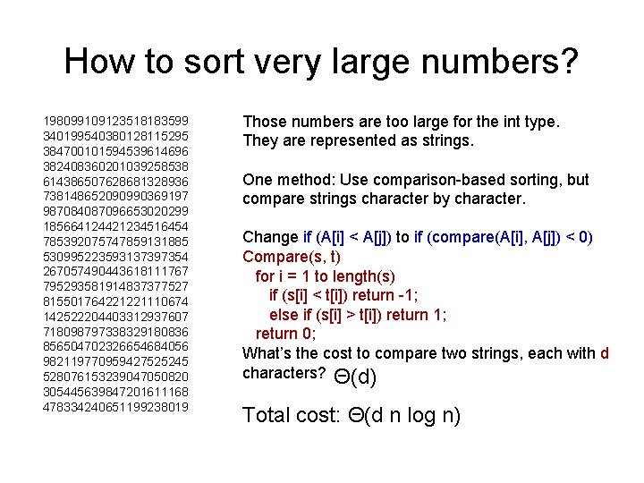
How to sort very large numbers? 198099109123518183599 340199540380128115295 384700101594539614696 382408360201039258538 614386507628681328936 738148652090990369197 987084087096653020299 185664124421234516454 785392075747859131885 530995223593137397354 267057490443618111767 795293581914837377527 815501764221221110674 142522204403312937607 718098797338329180836 856504702326654684056 982119770959427525245 528076153239047050820 305445639847201611168 478334240651199238019 Those numbers are too large for the int type. They are represented as strings. One method: Use comparison-based sorting, but compare strings character by character. Change if (A[i] < A[j]) to if (compare(A[i], A[j]) < 0) Compare(s, t) for i = 1 to length(s) if (s[i] < t[i]) return -1; else if (s[i] > t[i]) return 1; return 0; What’s the cost to compare two strings, each with d characters? Θ(d) Total cost: Θ(d n log n)

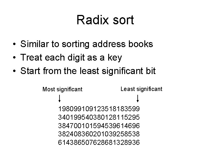
Radix sort • Similar to sorting address books • Treat each digit as a key • Start from the least significant bit Most significant Least significant 198099109123518183599 340199540380128115295 384700101594539614696 382408360201039258538 614386507628681328936

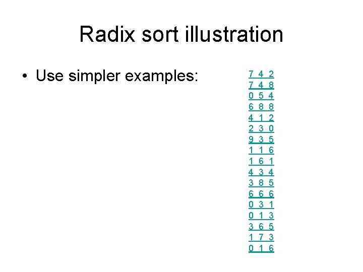
Radix sort illustration • Use simpler examples: 7 7 0 6 4 2 9 1 1 4 3 6 0 0 3 1 0 4 4 5 8 1 3 3 1 6 3 8 6 3 1 6 7 1 2 8 4 8 2 0 5 6 1 4 5 6 1 3 5 3 6

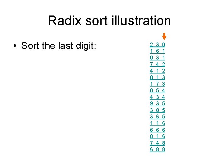
Radix sort illustration • Sort the last digit: 2 1 0 7 4 0 1 0 4 9 3 3 1 6 0 7 6 3 4 1 1 7 5 3 3 8 6 1 4 8 0 1 1 2 2 3 3 4 4 5 5 5 6 6 6 8 8

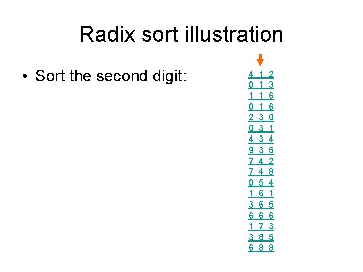
Radix sort illustration • Sort the second digit: 4 0 1 0 2 0 4 9 7 7 0 1 3 6 1 1 3 3 4 4 5 6 6 6 7 8 8 2 3 6 6 0 1 4 5 2 8 4 1 5 6 3 5 8

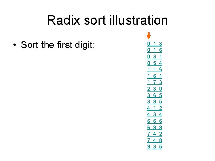
Radix sort illustration • Sort the first digit: 0 0 1 1 1 2 3 3 4 4 6 6 7 7 9 1 1 3 5 1 6 7 3 6 8 1 3 6 8 4 4 3 3 6 1 4 6 1 3 0 5 5 2 4 6 8 2 8 5

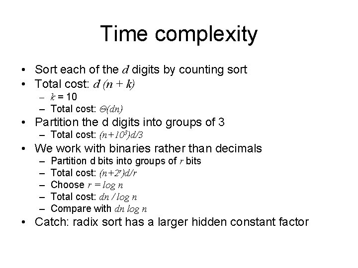
Time complexity • Sort each of the d digits by counting sort • Total cost: d (n + k) – k = 10 – Total cost: Θ(dn) • Partition the d digits into groups of 3 – Total cost: (n+103)d/3 • We work with binaries rather than decimals – – – Partition d bits into groups of r bits Total cost: (n+2 r)d/r Choose r = log n Total cost: dn / log n Compare with dn log n • Catch: radix sort has a larger hidden constant factor

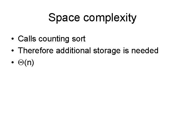
Space complexity • Calls counting sort • Therefore additional storage is needed • (n)