CS 3343 Analysis of Algorithms Lecture 17 Intro

CS 3343: Analysis of Algorithms Lecture 17: Intro to Dynamic Programming

In the next few lectures • Two important algorithm design techniques – Dynamic programming – Greedy algorithm • Meta algorithms, not actual algorithms (like divide-and-conquer) • Very useful in practice • Once you understand them, it is often easier to reinvent certain algorithms than trying to look them up!

Optimization Problems • An important and practical class of computational problems. – For each problem instance, there are many feasible solutions (often exponential) – Each solution has a value (or cost) – The goal is to find a solution with the optimal value • For most of these, the best known algorithm runs in exponential time. • Industry would pay dearly to have faster algorithms. • For some of them, there are quick dynamic programming or greedy algorithms. • For the rest, you may have to consider acceptable solutions rather than optimal solutions

Dynamic programming • The word “programming” is historical and predates computer programming • A very powerful, general tool for solving certain optimization problems • Once understood it is relatively easy to apply. • It looks like magic until you have seen enough examples

A motivating example: Fibonacci numbers • 1, 1, 2, 3, 5, 8, 13, 21, 34, 55, 89, … F(0) = 1; F(1) = 1; F(n) = F(n-1) + f(n-2) • How to compute F(n)?

A recursive algorithm function fib(n) if (n == 0 or n == 1) return 1; else return fib(n-1) + fib(n-2); What’s the time complexity?

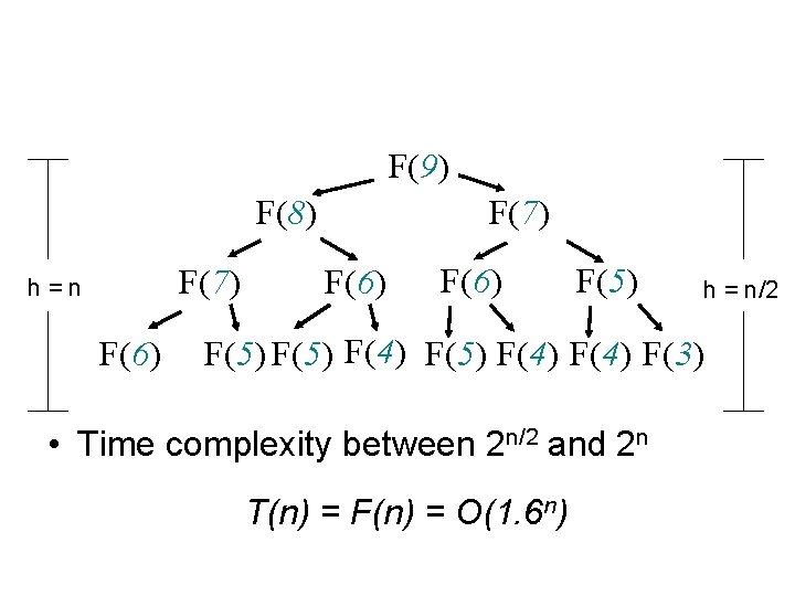
F(9) F(8) F(7) h=n F(6) F(7) F(6) F(5) h = n/2 F(5) F(4) F(3) • Time complexity between 2 n/2 and 2 n T(n) = F(n) = O(1. 6 n)

An iterative algorithm function fib(n) F[0] = 1; F[1] = 1; for i = 2 to n F[i] = F[i-1] + F[i-2]; Return F[n]; Time complexity?

• Problem with the recursive Fib algorithm: – Each subproblem was solved for many times! • Solution: avoid solving the same subproblem more than once (1) pre-compute all subproblems that may be needed later (2) Compute on demand, but memorize the solution to avoid recomputing • Can you always speedup a recursive algorithm by making it an iterative algorithm? – E. g. , merge sort – No. since there is no overlap between the two sub-problems

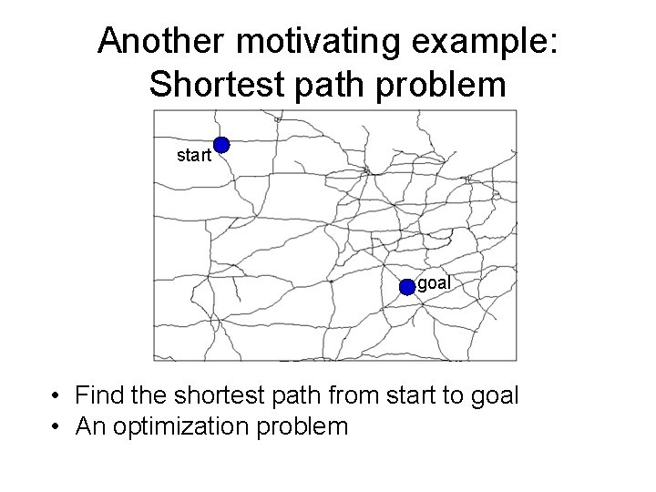
Another motivating example: Shortest path problem start goal • Find the shortest path from start to goal • An optimization problem

Possible approaches • Brute-force algorithm – Enumerate all possible paths and compare – How many? • Greedy algorithm – Always use the currently shortest edge – Does not necessarily lead to the optimal solution • Can you think about a recursive strategy?

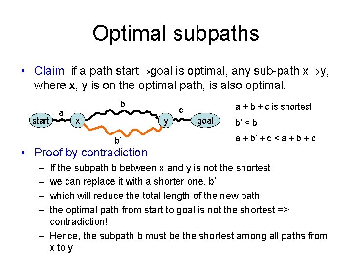
Optimal subpaths • Claim: if a path start goal is optimal, any sub-path x y, where x, y is on the optimal path, is also optimal. start a b x y b’ a + b + c is shortest c goal b’ < b a + b’ + c < a + b + c • Proof by contradiction – – If the subpath b between x and y is not the shortest we can replace it with a shorter one, b’ which will reduce the total length of the new path the optimal path from start to goal is not the shortest => contradiction! – Hence, the subpath b must be the shortest among all paths from x to y

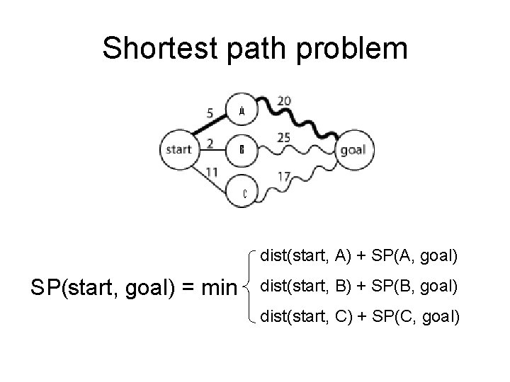
Shortest path problem dist(start, A) + SP(A, goal) SP(start, goal) = min dist(start, B) + SP(B, goal) dist(start, C) + SP(C, goal)

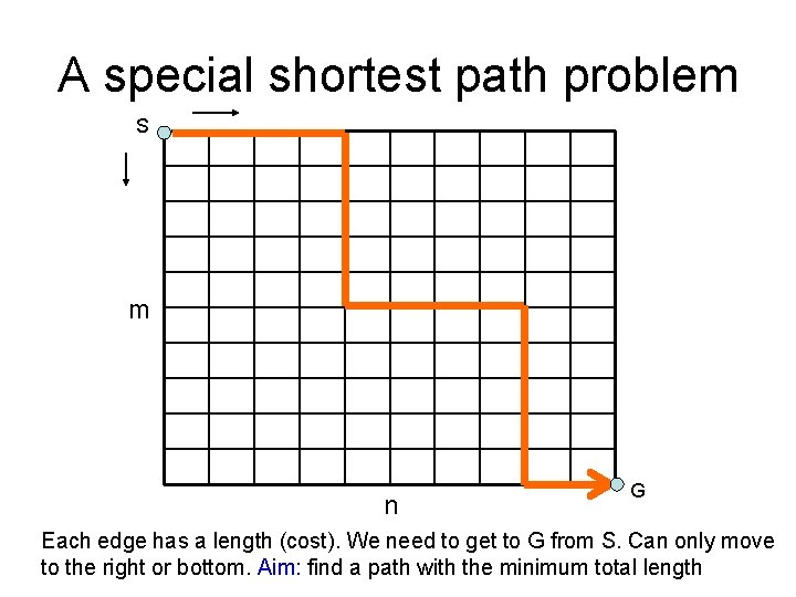
A special shortest path problem S m n G Each edge has a length (cost). We need to get to G from S. Can only move to the right or bottom. Aim: find a path with the minimum total length

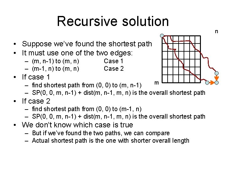
Recursive solution • Suppose we’ve found the shortest path • It must use one of the two edges: – (m, n-1) to (m, n) – (m-1, n) to (m, n) Case 1 Case 2 • If case 1 m – find shortest path from (0, 0) to (m, n-1) – SP(0, 0, m, n-1) + dist(m, n-1, m, n) is the overall shortest path • If case 2 – find shortest path from (0, 0) to (m-1, n) – SP(0, 0, m, n-1) + dist(m, n-1, m, n) is the overall shortest path • We don’t know which case is true – But if we’ve found the two paths, we can compare – Actual shortest path is the one with shorter overall length n

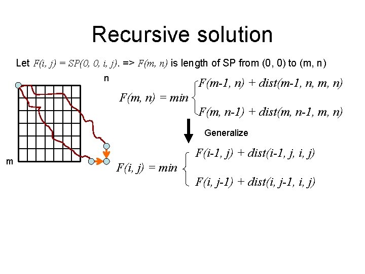
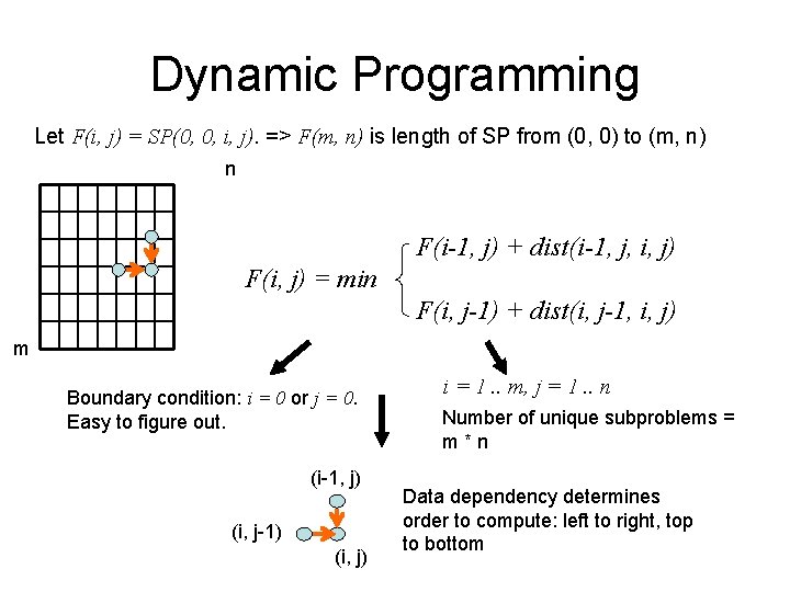
Recursive solution Let F(i, j) = SP(0, 0, i, j). => F(m, n) is length of SP from (0, 0) to (m, n) n F(m-1, n) + dist(m-1, n, m, n) F(m, n) = min F(m, n-1) + dist(m, n-1, m, n) Generalize m F(i-1, j) + dist(i-1, j, i, j) F(i, j) = min F(i, j-1) + dist(i, j-1, i, j)

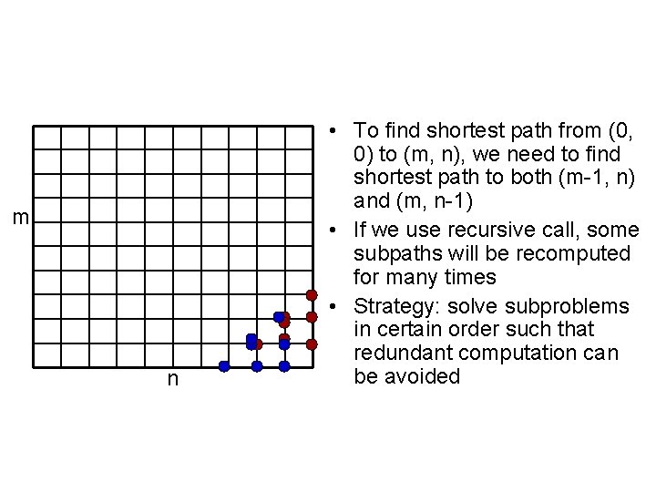
m n • To find shortest path from (0, 0) to (m, n), we need to find shortest path to both (m-1, n) and (m, n-1) • If we use recursive call, some subpaths will be recomputed for many times • Strategy: solve subproblems in certain order such that redundant computation can be avoided

Dynamic Programming Let F(i, j) = SP(0, 0, i, j). => F(m, n) is length of SP from (0, 0) to (m, n) n F(i-1, j) + dist(i-1, j, i, j) F(i, j) = min F(i, j-1) + dist(i, j-1, i, j) m Boundary condition: i = 0 or j = 0. Easy to figure out. (i-1, j) (i, j-1) (i, j) i = 1. . m, j = 1. . n Number of unique subproblems = m*n Data dependency determines order to compute: left to right, top to bottom

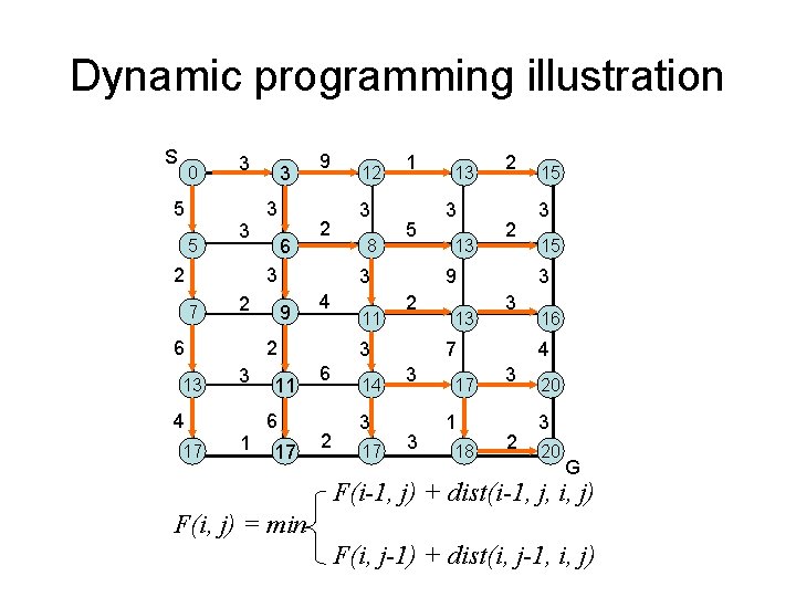
Dynamic programming illustration S 0 5 5 3 3 2 3 3 6 9 2 3 7 2 6 13 4 17 1 3 8 1 5 3 9 4 2 3 12 11 6 17 11 2 14 3 17 3 13 2 2 9 2 3 6 13 13 3 17 1 18 3 15 3 3 7 3 15 16 4 3 2 20 3 20 G F(i-1, j) + dist(i-1, j, i, j) F(i, j) = min F(i, j-1) + dist(i, j-1, i, j)

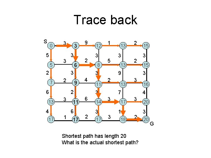
Trace back S 0 5 5 3 3 2 3 3 6 9 2 3 7 2 6 13 4 17 1 3 8 1 5 3 9 4 2 3 12 11 6 17 11 2 14 3 17 3 13 2 2 9 2 3 6 13 13 3 17 1 18 3 15 3 3 7 3 15 16 4 3 2 Shortest path has length 20 What is the actual shortest path? 20 3 20 G

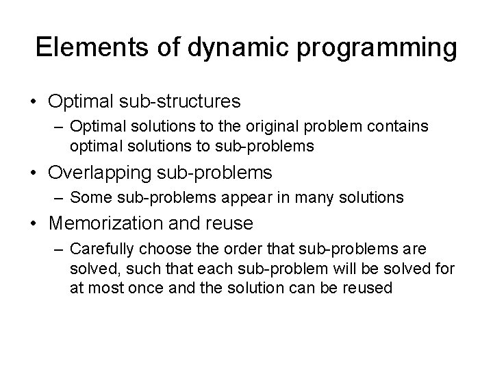
Elements of dynamic programming • Optimal sub-structures – Optimal solutions to the original problem contains optimal solutions to sub-problems • Overlapping sub-problems – Some sub-problems appear in many solutions • Memorization and reuse – Carefully choose the order that sub-problems are solved, such that each sub-problem will be solved for at most once and the solution can be reused

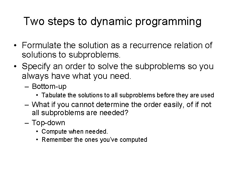
Two steps to dynamic programming • Formulate the solution as a recurrence relation of solutions to subproblems. • Specify an order to solve the subproblems so you always have what you need. – Bottom-up • Tabulate the solutions to all subproblems before they are used – What if you cannot determine the order easily, of if not all subproblems are needed? – Top-down • Compute when needed. • Remember the ones you’ve computed

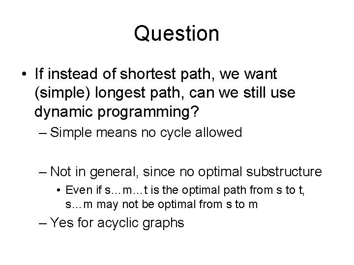
Question • If instead of shortest path, we want (simple) longest path, can we still use dynamic programming? – Simple means no cycle allowed – Not in general, since no optimal substructure • Even if s…m…t is the optimal path from s to t, s…m may not be optimal from s to m – Yes for acyclic graphs

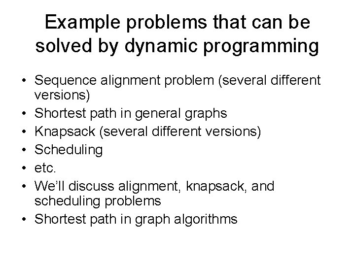
Example problems that can be solved by dynamic programming • Sequence alignment problem (several different versions) • Shortest path in general graphs • Knapsack (several different versions) • Scheduling • etc. • We’ll discuss alignment, knapsack, and scheduling problems • Shortest path in graph algorithms

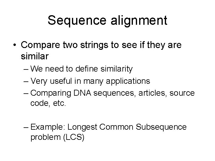
Sequence alignment • Compare two strings to see if they are similar – We need to define similarity – Very useful in many applications – Comparing DNA sequences, articles, source code, etc. – Example: Longest Common Subsequence problem (LCS)

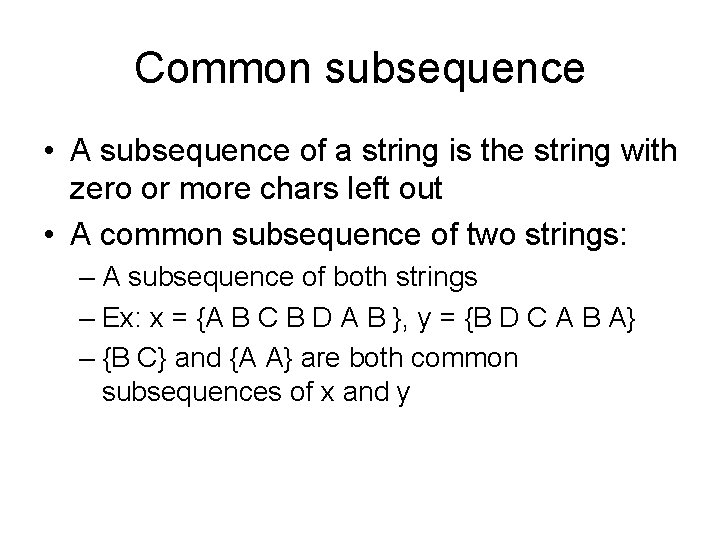
Common subsequence • A subsequence of a string is the string with zero or more chars left out • A common subsequence of two strings: – A subsequence of both strings – Ex: x = {A B C B D A B }, y = {B D C A B A} – {B C} and {A A} are both common subsequences of x and y

Longest Common Subsequence • Given two sequences x[1. . m] and y[1. . n], find a longest subsequence common to them both. “a” not “the” x: A B C B D A y: B D C A B BCBA = LCS(x, y) functional notation, but not a function

Brute-force LCS algorithm Check every subsequence of x[1. . m] to see if it is also a subsequence of y[1. . n]. Analysis • 2 m subsequences of x (each bit-vector of length m determines a distinct subsequence of x). • Hence, the runtime would be exponential ! Towards a better algorithm: a DP strategy • Key: optimal substructure and overlapping subproblems • First we’ll find the length of LCS. Later we’ll modify the algorithm to find LCS itself.

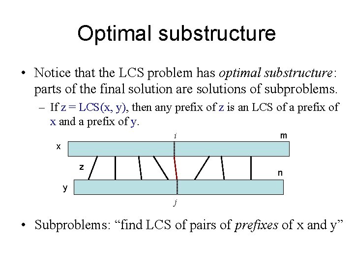
Optimal substructure • Notice that the LCS problem has optimal substructure: parts of the final solution are solutions of subproblems. – If z = LCS(x, y), then any prefix of z is an LCS of a prefix of x and a prefix of y. i m x z n y j • Subproblems: “find LCS of pairs of prefixes of x and y”

Recursive thinking m x n y • Case 1: x[m]=y[n]. There is an optimal LCS that matches x[m] with y[n]. Find out LCS (x[1. . m-1], y[1. . n-1]) • Case 2: x[m] y[n]. At most one of them is in LCS – Case 2. 1: x[m] not in LCS – Case 2. 2: y[n] not in LCS Find out LCS (x[1. . m-1], y[1. . n]) Find out LCS (x[1. . m], y[1. . n-1])

Recursive thinking m x n y • Case 1: x[m]=y[n] Reduce both sequences by 1 char – LCS(x, y) = LCS(x[1. . m-1], y[1. . n-1]) || x[m] • Case 2: x[m] y[n] concatenate – LCS(x, y) = LCS(x[1. . m-1], y[1. . n]) or LCS(x[1. . m], y[1. . n-1]), whichever is longer Reduce either sequence by 1 char

Finding length of LCS m x n y • Let c[i, j] be the length of LCS(x[1. . i], y[1. . j]) => c[m, n] is the length of LCS(x, y) • If x[m] = y[n] c[m, n] = c[m-1, n-1] + 1 • If x[m] != y[n] c[m, n] = max { c[m-1, n], c[m, n-1] }

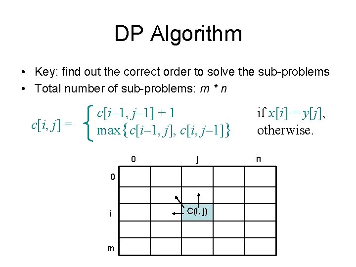
Generalize: recursive formulation c[i– 1, j– 1] + 1 max{c[i– 1, j], c[i, j– 1]} c[i, j] = 1 2 i m . . . x: 1 y: if x[i] = y[j], otherwise. 2 j n . . .

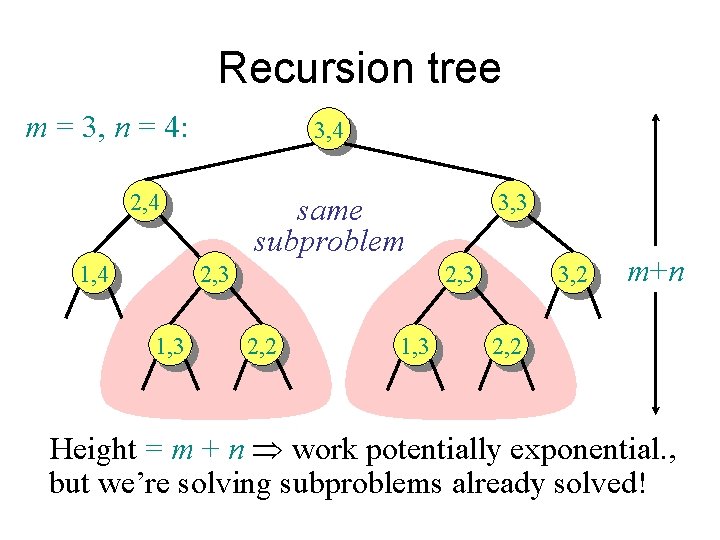
Recursive algorithm for LCS(x, y, i, j) if x[i] = y[ j] then c[i, j] LCS(x, y, i– 1, j– 1) + 1 else c[i, j] max{ LCS(x, y, i– 1, j), LCS(x, y, i, j– 1)} Worst-case: x[i] ¹ y[ j], in which case the algorithm evaluates two subproblems, each with only one parameter decremented.

Recursion tree m = 3, n = 4: 3, 4 2, 4 1, 4 2, 3 1, 3 3, 3 same subproblem 3, 2 2, 3 2, 2 1, 3 m+n 2, 2 Height = m + n work potentially exponential. , but we’re solving subproblems already solved!

DP Algorithm • Key: find out the correct order to solve the sub-problems • Total number of sub-problems: m * n c[i, j] = c[i– 1, j– 1] + 1 max{c[i– 1, j], c[i, j– 1]} 0 j 0 i m C(i, j) if x[i] = y[j], otherwise. n

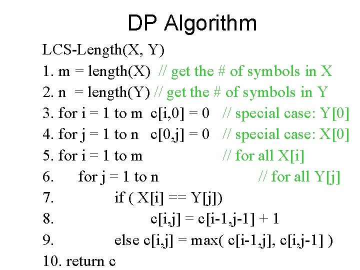
DP Algorithm LCS-Length(X, Y) 1. m = length(X) // get the # of symbols in X 2. n = length(Y) // get the # of symbols in Y 3. for i = 1 to m c[i, 0] = 0 // special case: Y[0] 4. for j = 1 to n c[0, j] = 0 // special case: X[0] 5. for i = 1 to m // for all X[i] 6. for j = 1 to n // for all Y[j] 7. if ( X[i] == Y[j]) 8. c[i, j] = c[i-1, j-1] + 1 9. else c[i, j] = max( c[i-1, j], c[i, j-1] ) 10. return c

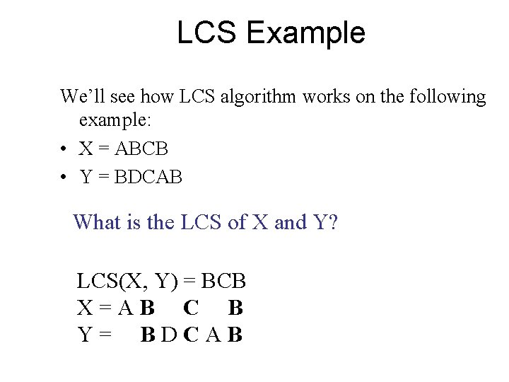
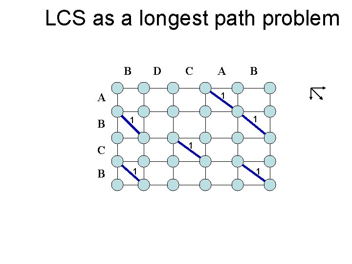
LCS Example We’ll see how LCS algorithm works on the following example: • X = ABCB • Y = BDCAB What is the LCS of X and Y? LCS(X, Y) = BCB X=AB C B Y= BDCAB

LCS Example (0) j i 0 X[i] 1 A 2 B 3 C 4 B 0 Y[j] 1 B 2 D X = ABCB; m = |X| = 4 Y = BDCAB; n = |Y| = 5 Allocate array c[5, 6] 3 C 4 A ABCB BDCAB 5 B

LCS Example (1) j i ABCB BDCAB 5 0 Y[j] 1 B 2 D 3 C 4 A B 0 0 0 X[i] 0 1 A 0 2 B 0 3 C 0 4 B 0 for i = 1 to m for j = 1 to n c[i, 0] = 0 c[0, j] = 0

LCS Example (2) j i ABCB BDCAB 5 0 Y[j] 1 B 2 D 3 C 4 A B 0 0 0 X[i] 0 0 1 A 0 0 2 B 0 3 C 0 4 B 0 if ( Xi == Yj ) c[i, j] = c[i-1, j-1] + 1 else c[i, j] = max( c[i-1, j], c[i, j-1] )

LCS Example (3) j i ABCB BDCAB 5 0 Y[j] 1 B 2 D 3 C 4 A B 0 0 0 X[i] 0 0 1 A 0 0 2 B 0 3 C 0 4 B 0 if ( Xi == Yj ) c[i, j] = c[i-1, j-1] + 1 else c[i, j] = max( c[i-1, j], c[i, j-1] )

LCS Example (4) j i ABCB BDCAB 5 0 Y[j] 1 B 2 D 3 C 4 A B 0 0 X[i] 0 0 0 1 A 0 0 1 2 B 0 3 C 0 4 B 0 if ( Xi == Yj ) c[i, j] = c[i-1, j-1] + 1 else c[i, j] = max( c[i-1, j], c[i, j-1] )

LCS Example (5) j i ABCB BDCAB 5 0 Y[j] 1 B 2 D 3 C 4 A B 0 X[i] 0 0 0 1 A 0 0 1 1 2 B 0 3 C 0 4 B 0 if ( Xi == Yj ) c[i, j] = c[i-1, j-1] + 1 else c[i, j] = max( c[i-1, j], c[i, j-1] )

LCS Example (6) j i ABCB BDCAB 5 0 Y[j] 1 B 2 D 3 C 4 A B 0 X[i] 0 0 0 1 A 0 0 1 1 2 B 0 1 3 C 0 4 B 0 if ( Xi == Yj ) c[i, j] = c[i-1, j-1] + 1 else c[i, j] = max( c[i-1, j], c[i, j-1] )

LCS Example (7) j i ABCB BDCAB 5 0 Y[j] 1 B 2 D 3 C 4 A B 0 X[i] 0 0 0 1 A 0 0 1 1 2 B 0 1 1 3 C 0 4 B 0 if ( Xi == Yj ) c[i, j] = c[i-1, j-1] + 1 else c[i, j] = max( c[i-1, j], c[i, j-1] )

LCS Example (8) j i ABCB BDCAB 5 0 Y[j] 1 B 2 D 3 C 4 A B 0 X[i] 0 0 0 1 A 0 0 1 1 2 B 0 1 1 2 3 C 0 4 B 0 if ( Xi == Yj ) c[i, j] = c[i-1, j-1] + 1 else c[i, j] = max( c[i-1, j], c[i, j-1] )

LCS Example (9) j i ABCB BDCAB 5 0 Y[j] 1 B 2 D 3 C 4 A B 0 X[i] 0 0 0 1 A 0 0 1 1 2 B 0 1 1 2 3 C 0 1 1 4 B 0 if ( Xi == Yj ) c[i, j] = c[i-1, j-1] + 1 else c[i, j] = max( c[i-1, j], c[i, j-1] )

LCS Example (10) j i ABCB BDCAB 5 0 Y[j] 1 B 2 D 3 C 4 A B 0 X[i] 0 0 0 1 A 0 0 1 1 2 B 0 1 1 2 3 C 0 1 1 2 4 B 0 if ( Xi == Yj ) c[i, j] = c[i-1, j-1] + 1 else c[i, j] = max( c[i-1, j], c[i, j-1] )

LCS Example (11) j i ABCB BDCAB 5 0 Y[j] 1 B 2 D 3 C 4 A B 0 X[i] 0 0 0 1 A 0 0 1 1 2 B 0 1 1 2 3 C 0 1 1 2 2 2 4 B 0 if ( Xi == Yj ) c[i, j] = c[i-1, j-1] + 1 else c[i, j] = max( c[i-1, j], c[i, j-1] )

LCS Example (12) j i ABCB BDCAB 5 0 Y[j] 1 B 2 D 3 C 4 A B 0 X[i] 0 0 0 1 A 0 0 1 1 2 B 0 1 1 2 3 C 0 1 1 2 2 2 4 B 0 1 if ( Xi == Yj ) c[i, j] = c[i-1, j-1] + 1 else c[i, j] = max( c[i-1, j], c[i, j-1] )

LCS Example (13) j i ABCB BDCAB 5 0 Y[j] 1 B 2 D 3 C 4 A B 0 X[i] 0 0 0 1 A 0 0 1 1 2 B 0 1 1 2 3 C 0 1 1 2 2 2 4 B 0 1 1 2 2 if ( Xi == Yj ) c[i, j] = c[i-1, j-1] + 1 else c[i, j] = max( c[i-1, j], c[i, j-1] )

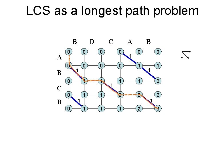
LCS Example (14) j i ABCB BDCAB 5 0 Y[j] 1 B 2 D 3 C 4 A B 0 X[i] 0 0 0 1 A 0 0 1 1 2 B 0 1 1 2 3 C 0 1 1 2 2 2 4 B 0 1 1 2 2 3 if ( Xi == Yj ) c[i, j] = c[i-1, j-1] + 1 else c[i, j] = max( c[i-1, j], c[i, j-1] )

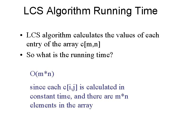
LCS Algorithm Running Time • LCS algorithm calculates the values of each entry of the array c[m, n] • So what is the running time? O(m*n) since each c[i, j] is calculated in constant time, and there are m*n elements in the array

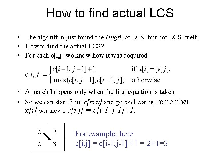
How to find actual LCS • The algorithm just found the length of LCS, but not LCS itself. • How to find the actual LCS? • For each c[i, j] we know how it was acquired: • A match happens only when the first equation is taken • So we can start from c[m, n] and go backwards, remember x[i] whenever c[i, j] = c[i-1, j-1]+1. 2 2 2 3 For example, here c[i, j] = c[i-1, j-1] +1 = 2+1=3

Finding LCS j 0 Y[j] 1 B 2 D 3 C 4 A 5 B 0 X[i] 0 0 0 1 A 0 0 1 1 2 B 0 1 1 2 3 C 0 1 1 2 2 2 4 B 0 1 1 2 2 3 i Time for trace back: O(m+n).

Finding LCS (2) j 0 Y[j] 1 B 2 D 3 C 4 A 5 B 0 X[i] 0 0 0 1 A 0 0 1 1 2 B 0 1 1 2 3 C 0 1 1 2 2 2 4 B 0 1 1 2 2 3 i LCS (reversed order): B C B LCS (straight order): B C B (this string turned out to be a palindrome)

LCS as a longest path problem B D C A B B 1 1 C B A 1 1

LCS as a longest path problem B A D C A 0 0 0 0 1 1 B 1 C 1 B 0 0 0 1 1 2 2 1 1 B 0 1 1 1 2 3

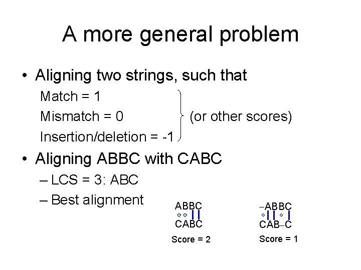
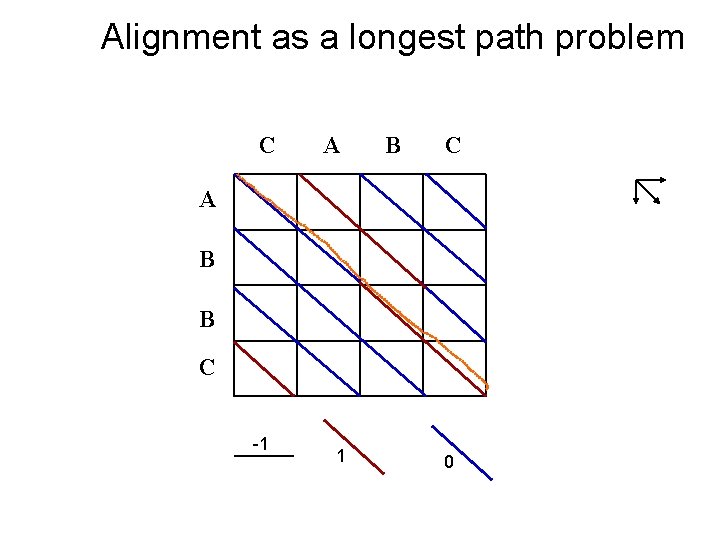
A more general problem • Aligning two strings, such that Match = 1 Mismatch = 0 Insertion/deletion = -1 (or other scores) • Aligning ABBC with CABC – LCS = 3: ABC – Best alignment ABBC CABC CAB C Score = 2 Score = 1

• Let F(i, j) be the best alignment score between X[1. . i] and Y[1. . j]. • F(m, n) is the best alignment score between X and Y • Recurrence F(i-1, j-1) + (i, j) Match/Mismatch F(i, j) = max F(i-1, j) – 1 F(i, j-1) – 1 Insertion on Y Insertion on X (i, j) = 1 if X[i]=Y[j] and 0 otherwise.

Alignment Example j i 0 X[i] 1 A 2 B 3 B 4 C 0 Y[j] 1 C 2 A X = ABBC; m = |X| = 4 Y = CABC; n = |Y| = 4 Allocate array F[5, 5] 3 B 4 C ABBC CABC

Alignment Example j i 0 X[i] 0 Y[j] 1 C 2 A 3 B 4 C 0 -1 -2 -3 -4 1 A -1 0 0 -1 -2 2 B -2 -1 0 3 B -3 -2 -1 1 1 4 C -4 -2 -2 0 2 F(i-1, j-1) + (i, j) F(i, j) = max F(i-1, j) – 1 F(i, j-1) – 1 ABBC CABC Match/Mismatch Insertion on Y Insertion on X (i, j) = 1 if X[i]=Y[j] and 0 otherwise.

Alignment Example j i 0 X[i] 0 Y[j] 1 C 2 A 3 B 4 C 0 -1 -2 -3 -4 1 A -1 0 0 -1 -2 2 B -2 -1 0 3 B -3 -2 -1 1 1 4 C -4 -2 -2 0 2 ABBC CABC ABBC F(i-1, j-1) + (i, j) F(i, j) = max F(i-1, j) – 1 F(i, j-1) – 1 CABC Score = 2 Match/Mismatch Insertion on Y Insertion on X (i, j) = 1 if X[i]=Y[j] and 0 otherwise.

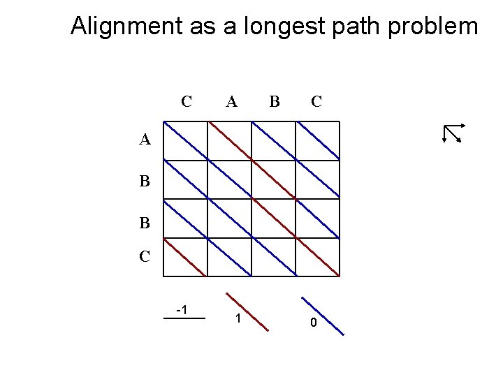
Alignment as a longest path problem C A B B C -1 1 0

Alignment as a longest path problem C A B B C -1 1 0