Numerical Integration Roger Crawfis Quadrature We talk in

Numerical Integration Roger Crawfis

Quadrature • We talk in terms of Quadrature Rules – 1. The process of making something square. 2. Mathematics The process of constructing a square equal in area to a given surface. 3. Astronomy A configuration in which the position of one celestial body is 90° from another celestial body, as measured from a third. – The American Heritage® Dictionary: Fourth Edition. 2000 16 September 2021 OSU/CSE 541 2

Outline • Definite Integrals • Lower and Upper Sums – Reimann Integration or Reimann Sums • Uniformly-spaced samples – – Trapezoid Rules Romberg Integration Simpson’s Rules Adaptive Simpson’s Scheme • Non-uniformly spaced samples – Gaussian Quadrature Formulas 16 September 2021 OSU/CSE 541 3

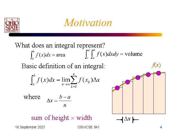
Motivation What does an integral represent? f(x) Basic definition of an integral: where sum of height width 16 September 2021 OSU/CSE 541 x 4

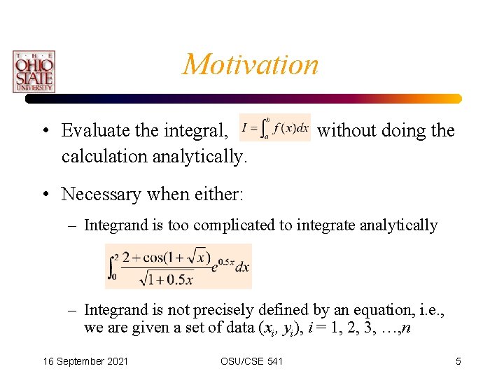
Motivation • Evaluate the integral, calculation analytically. without doing the • Necessary when either: – Integrand is too complicated to integrate analytically – Integrand is not precisely defined by an equation, i. e. , we are given a set of data (xi, yi), i = 1, 2, 3, …, n 16 September 2021 OSU/CSE 541 5

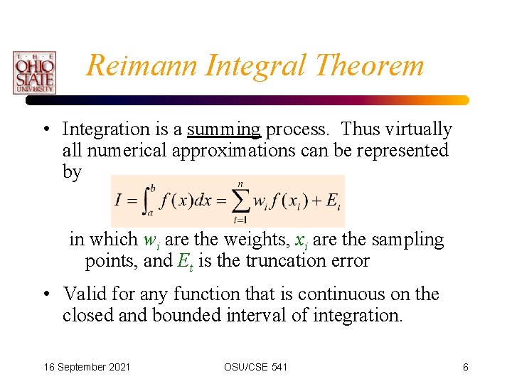
Reimann Integral Theorem • Integration is a summing process. Thus virtually all numerical approximations can be represented by in which wi are the weights, xi are the sampling points, and Et is the truncation error • Valid for any function that is continuous on the closed and bounded interval of integration. 16 September 2021 OSU/CSE 541 6

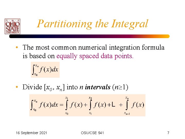
Partitioning the Integral • The most common numerical integration formula is based on equally spaced data points. • Divide [x 0 , xn] into n intervals (n 1) 16 September 2021 OSU/CSE 541 7

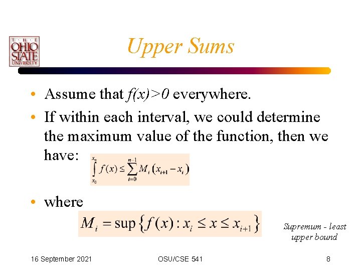
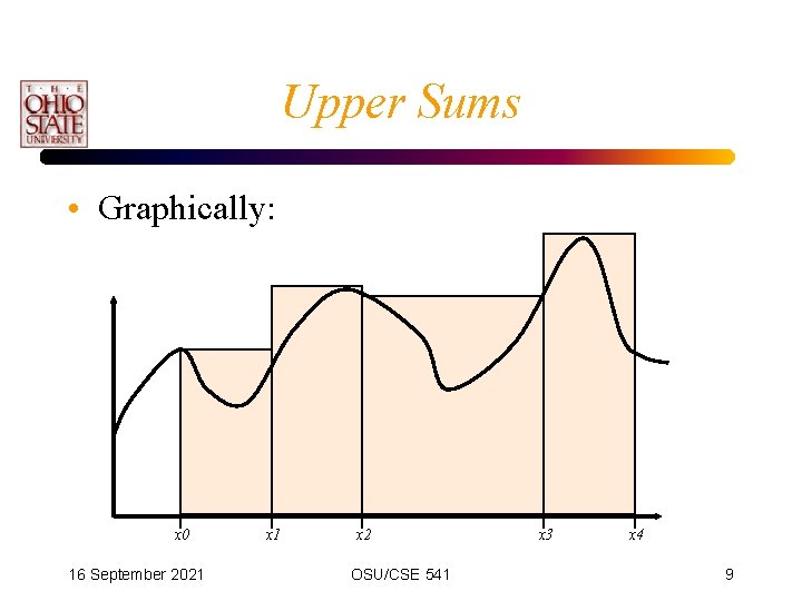
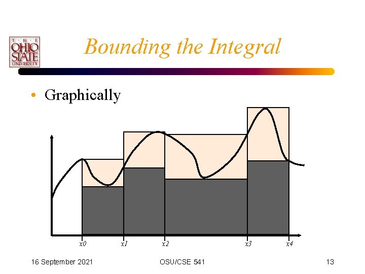
Upper Sums • Assume that f(x)>0 everywhere. • If within each interval, we could determine the maximum value of the function, then we have: • where Supremum - least upper bound 16 September 2021 OSU/CSE 541 8

Upper Sums • Graphically: x 0 16 September 2021 x 2 OSU/CSE 541 x 3 x 4 9

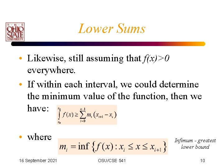
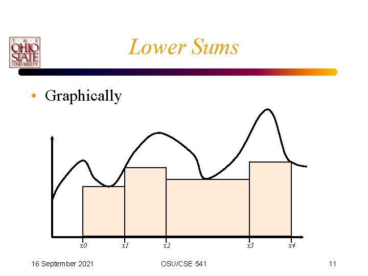
Lower Sums • Likewise, still assuming that f(x)>0 everywhere. • If within each interval, we could determine the minimum value of the function, then we have: • where 16 September 2021 Infimum - greatest lower bound OSU/CSE 541 10

Lower Sums • Graphically x 0 16 September 2021 x 2 OSU/CSE 541 x 3 x 4 11

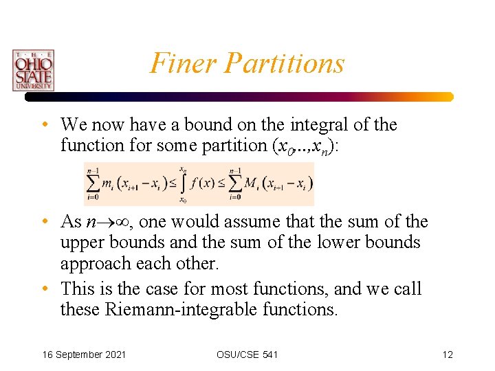
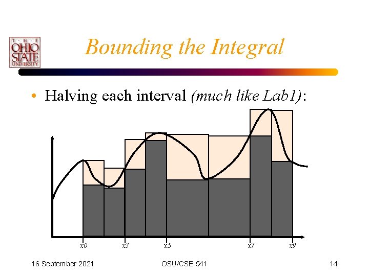
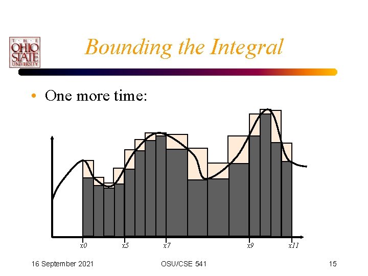
Finer Partitions • We now have a bound on the integral of the function for some partition (x 0, . . , xn): • As n , one would assume that the sum of the upper bounds and the sum of the lower bounds approach each other. • This is the case for most functions, and we call these Riemann-integrable functions. 16 September 2021 OSU/CSE 541 12

Bounding the Integral • Graphically x 0 16 September 2021 x 2 OSU/CSE 541 x 3 x 4 13

Bounding the Integral • Halving each interval (much like Lab 1): x 0 16 September 2021 x 3 x 5 OSU/CSE 541 x 7 x 9 14

Bounding the Integral • One more time: x 0 16 September 2021 x 5 x 7 OSU/CSE 541 x 9 x 11 15

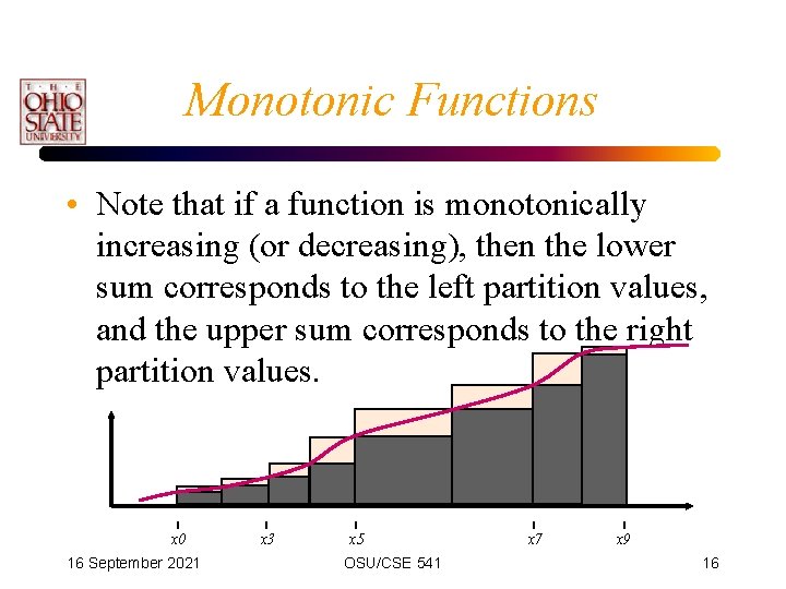
Monotonic Functions • Note that if a function is monotonically increasing (or decreasing), then the lower sum corresponds to the left partition values, and the upper sum corresponds to the right partition values. x 0 16 September 2021 x 3 x 5 OSU/CSE 541 x 7 x 9 16

Lab 1 and Integration • Thinking back to lab 1, what were the limits or the integration? • Is the sin function monotonic on this interval? • Should the Reiman sum be an upper or lower sum? 16 September 2021 OSU/CSE 541 17

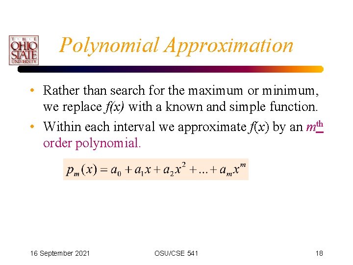
Polynomial Approximation • Rather than search for the maximum or minimum, we replace f(x) with a known and simple function. • Within each interval we approximate f(x) by an mth order polynomial. 16 September 2021 OSU/CSE 541 18

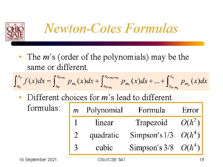
Newton-Cotes Formulas • The m’s (order of the polynomials) may be the same or different. • Different choices for m’s lead to different formulas: 16 September 2021 OSU/CSE 541 19

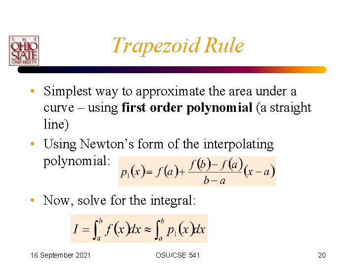
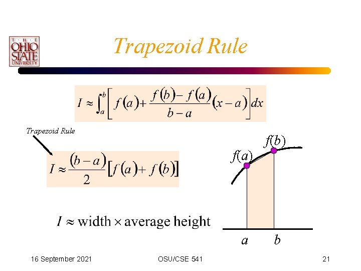
Trapezoid Rule • Simplest way to approximate the area under a curve – using first order polynomial (a straight line) • Using Newton’s form of the interpolating polynomial: • Now, solve for the integral: 16 September 2021 OSU/CSE 541 20

Trapezoid Rule f(a) a 16 September 2021 OSU/CSE 541 f(b) b 21

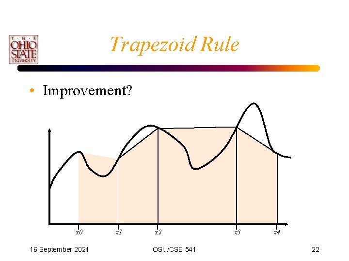
Trapezoid Rule • Improvement? x 0 16 September 2021 x 2 OSU/CSE 541 x 3 x 4 22

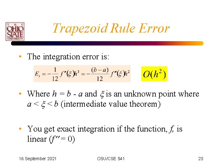
Trapezoid Rule Error • The integration error is: • Where h = b - a and is an unknown point where a < < b (intermediate value theorem) • You get exact integration if the function, f, is linear (f = 0) 16 September 2021 OSU/CSE 541 23

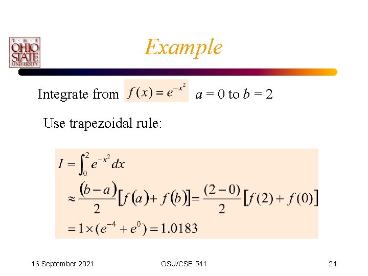
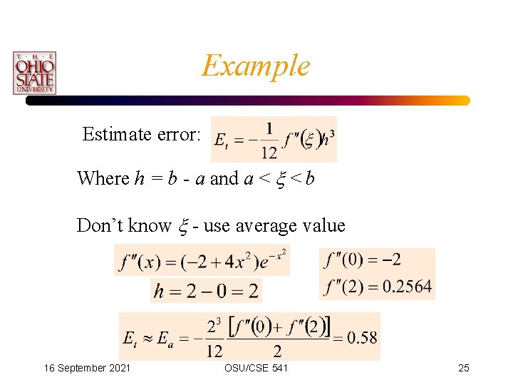
Example Integrate from a = 0 to b = 2 Use trapezoidal rule: 16 September 2021 OSU/CSE 541 24

Example Estimate error: Where h = b - a and a < < b Don’t know - use average value 16 September 2021 OSU/CSE 541 25

More intervals, better result [error O(h 2)] n=2 n=3 n=4 n=8 16 September 2021 OSU/CSE 541 26

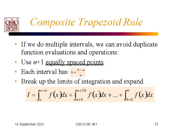
Composite Trapezoid Rule • If we do multiple intervals, we can avoid duplicate function evaluations and operations: • Use n+1 equally spaced points. • Each interval has: • Break up the limits of integration and expand. 16 September 2021 OSU/CSE 541 27

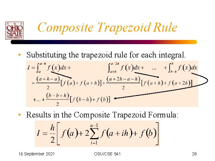
Composite Trapezoid Rule • Substituting the trapezoid rule for each integral. • Results in the Composite Trapezoid Formula: 16 September 2021 OSU/CSE 541 28

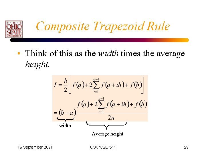
Composite Trapezoid Rule • Think of this as the width times the average height. width Average height 16 September 2021 OSU/CSE 541 29

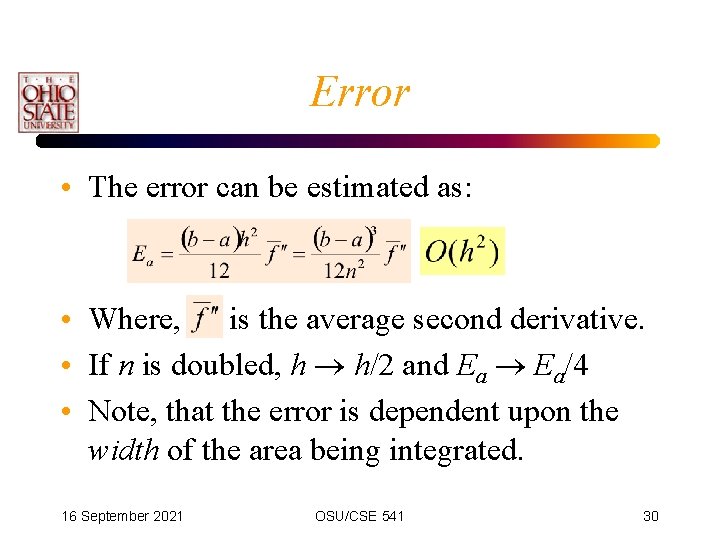
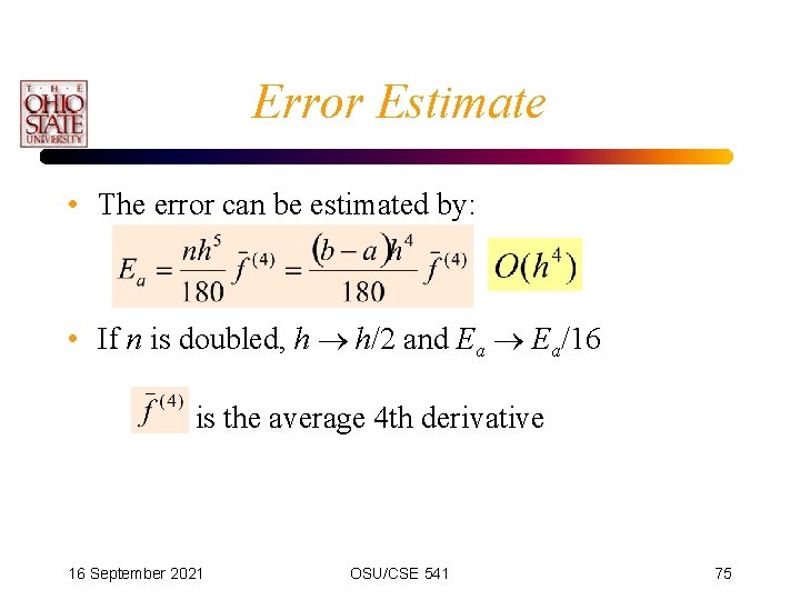
Error • The error can be estimated as: • Where, is the average second derivative. • If n is doubled, h h/2 and Ea Ea/4 • Note, that the error is dependent upon the width of the area being integrated. 16 September 2021 OSU/CSE 541 30

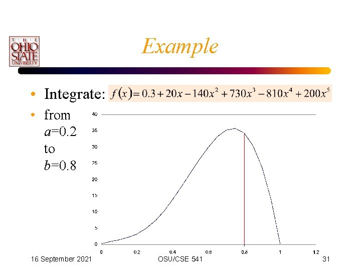
Example • Integrate: • from a=0. 2 to b=0. 8 16 September 2021 OSU/CSE 541 31

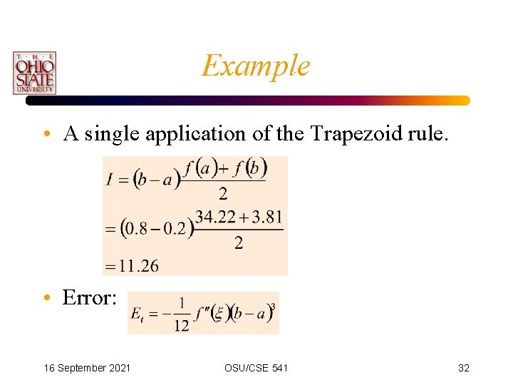
Example • A single application of the Trapezoid rule. • Error: 16 September 2021 OSU/CSE 541 32

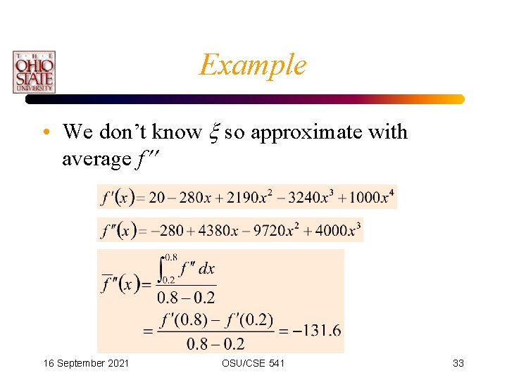
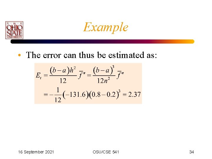
Example • We don’t know so approximate with average f 16 September 2021 OSU/CSE 541 33

Example • The error can thus be estimated as: 16 September 2021 OSU/CSE 541 34

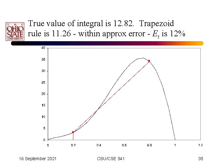
True value of integral is 12. 82. Trapezoid rule is 11. 26 - within approx error - Et is 12% 16 September 2021 OSU/CSE 541 35

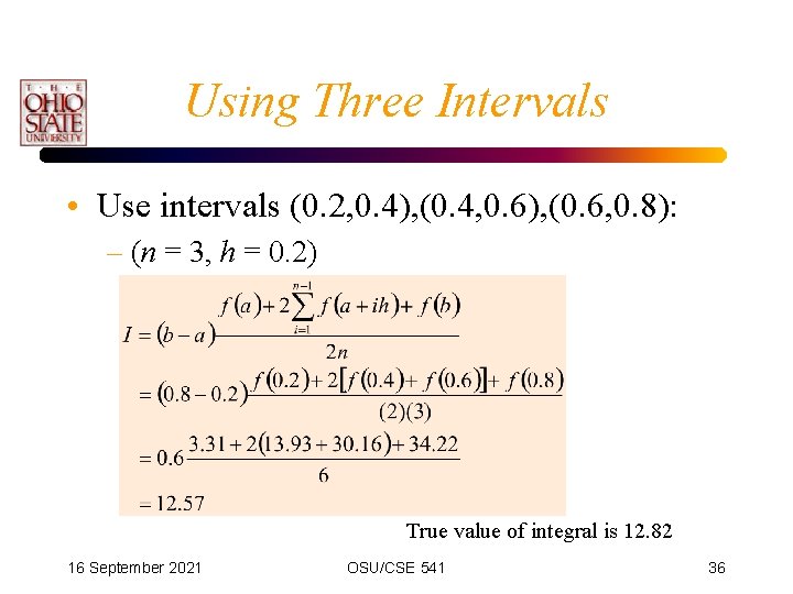
Using Three Intervals • Use intervals (0. 2, 0. 4), (0. 4, 0. 6), (0. 6, 0. 8): – (n = 3, h = 0. 2) True value of integral is 12. 82 16 September 2021 OSU/CSE 541 36

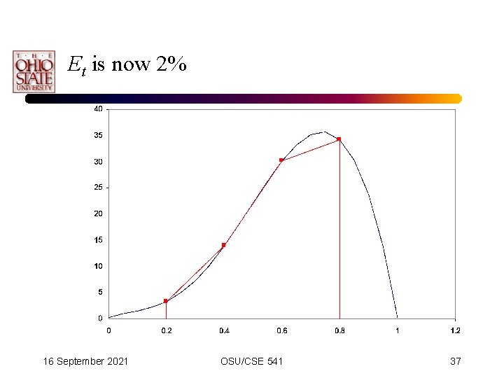
Et is now 2% 16 September 2021 OSU/CSE 541 37

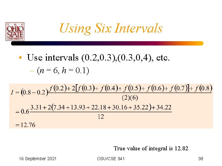
Using Six Intervals • Use intervals (0. 2, 0. 3), (0. 3, 0, 4), etc. – (n = 6, h = 0. 1) True value of integral is 12. 82 16 September 2021 OSU/CSE 541 38

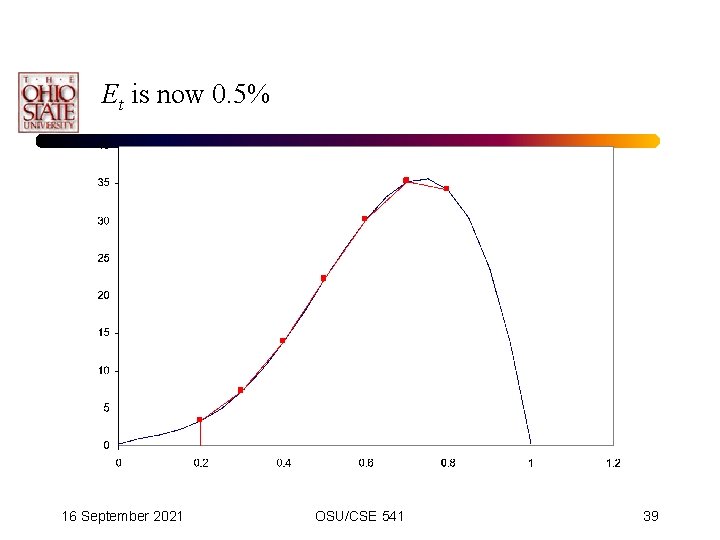
Et is now 0. 5% 16 September 2021 OSU/CSE 541 39

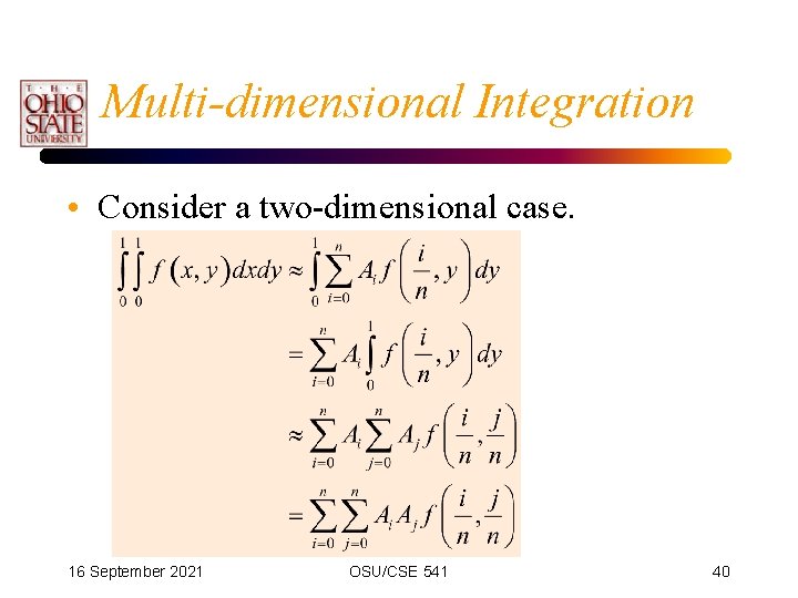
Multi-dimensional Integration • Consider a two-dimensional case. 16 September 2021 OSU/CSE 541 40

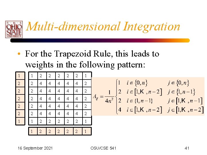
Multi-dimensional Integration • For the Trapezoid Rule, this leads to weights in the following pattern: 1 1 2 2 2 1 2 2 4 4 4 4 4 2 2 2 4 4 4 2 1 1 2 2 2 2 2 1 16 September 2021 OSU/CSE 541 41

Multi-dimensional Integration • If we use the weights from the Trapezoid rule, the error is still O(h 2). • However, there are now n 2 function evaluations. – Equally-spaced samples on a square region. 16 September 2021 OSU/CSE 541 42

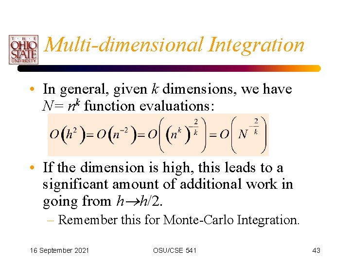
Multi-dimensional Integration • In general, given k dimensions, we have N= nk function evaluations: • If the dimension is high, this leads to a significant amount of additional work in going from h h/2. – Remember this for Monte-Carlo Integration. 16 September 2021 OSU/CSE 541 43

Reducing the Error • To improve the estimate of the integral, we can either: – Add more intervals – Use a higher order polynomial – Use Richardson Extrapolation to examine the limit as h 0. • Called Romberg Integration 16 September 2021 OSU/CSE 541 44

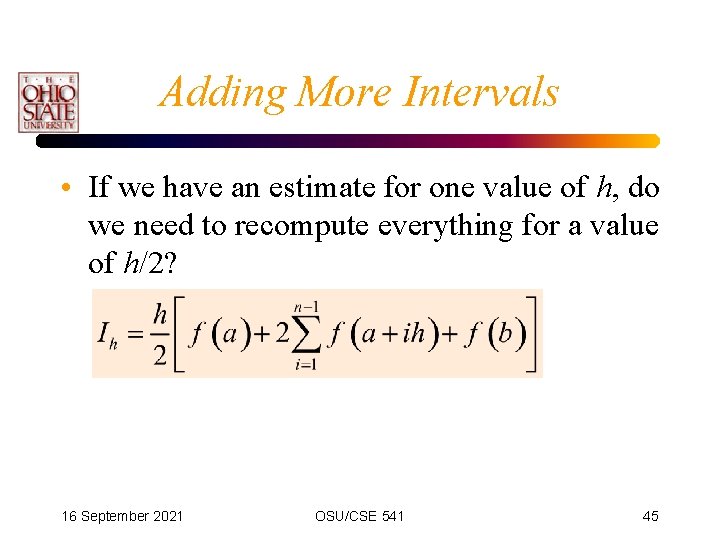
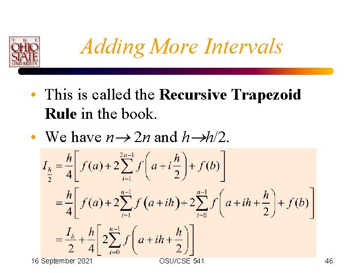
Adding More Intervals • If we have an estimate for one value of h, do we need to recompute everything for a value of h/2? 16 September 2021 OSU/CSE 541 45

Adding More Intervals • This is called the Recursive Trapezoid Rule in the book. • We have n 2 n and h h/2. 16 September 2021 OSU/CSE 541 46

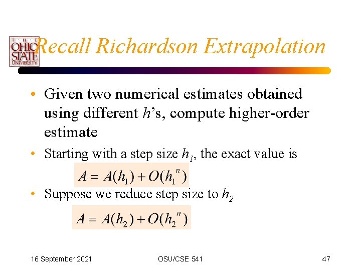
Recall Richardson Extrapolation • Given two numerical estimates obtained using different h’s, compute higher-order estimate • Starting with a step size h 1, the exact value is • Suppose we reduce step size to h 2 16 September 2021 OSU/CSE 541 47

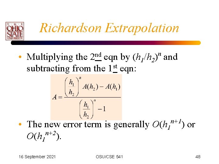
Richardson Extrapolation n • Multiplying the eqn by (h 1/h 2) and subtracting from the 1 st eqn: 2 nd • The new error term is generally O(h 1 n+1) or O(h 1 n+2). 16 September 2021 OSU/CSE 541 48

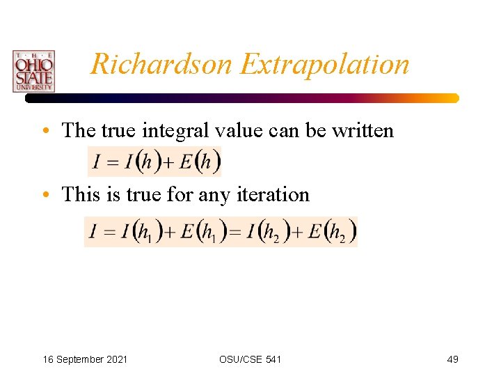
Richardson Extrapolation • The true integral value can be written • This is true for any iteration 16 September 2021 OSU/CSE 541 49

Richardson Extrapolation • For example: Using (n = 2) [error = O(h 2)] • where c is a constant • Therefore: 16 September 2021 OSU/CSE 541 order of error in trapezoidal rule 50

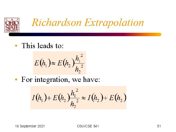
Richardson Extrapolation • This leads to: • For integration, we have: 16 September 2021 OSU/CSE 541 51

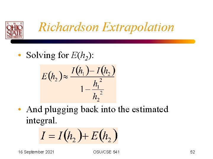
Richardson Extrapolation • Solving for E(h 2): • And plugging back into the estimated integral. 16 September 2021 OSU/CSE 541 52

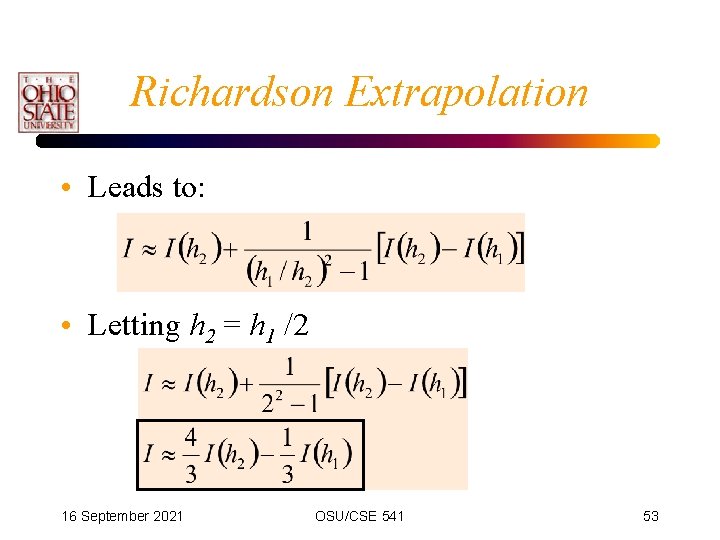
Richardson Extrapolation • Leads to: • Letting h 2 = h 1 /2 16 September 2021 OSU/CSE 541 53

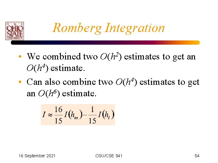
Romberg Integration • We combined two O(h 2) estimates to get an O(h 4) estimate. • Can also combine two O(h 4) estimates to get an O(h 6) estimate. 16 September 2021 OSU/CSE 541 54

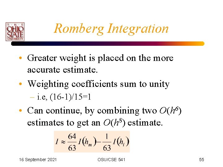
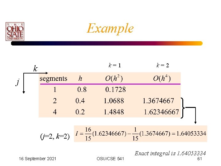
Romberg Integration • Greater weight is placed on the more accurate estimate. • Weighting coefficients sum to unity – i. e, (16 -1)/15=1 • Can continue, by combining two O(h 6) estimates to get an O(h 8) estimate. 16 September 2021 OSU/CSE 541 55

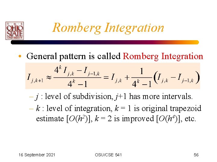
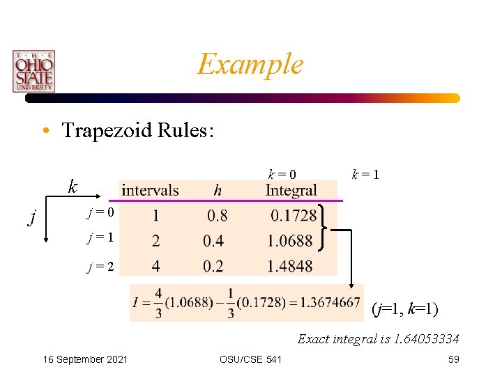
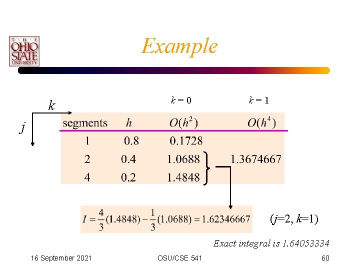
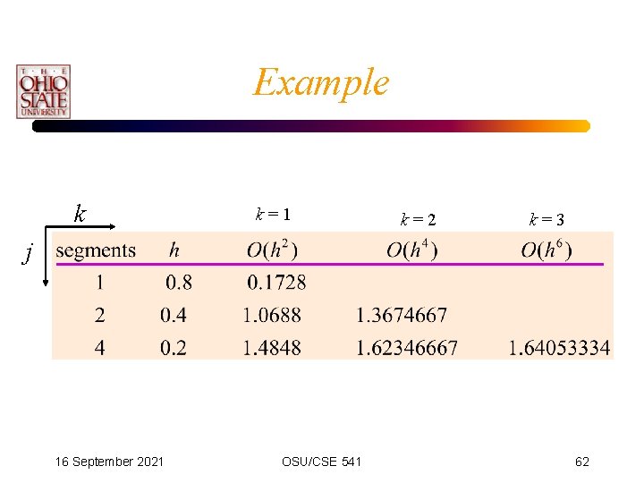
Romberg Integration • General pattern is called Romberg Integration – j : level of subdivision, j+1 has more intervals. – k : level of integration, k = 1 is original trapezoid estimate [O(h 2)], k = 2 is improved [O(h 4)], etc. 16 September 2021 OSU/CSE 541 56

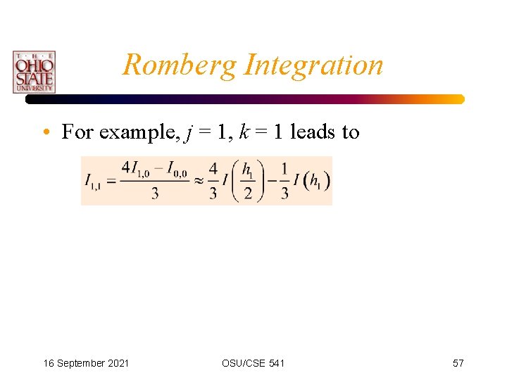
Romberg Integration • For example, j = 1, k = 1 leads to 16 September 2021 OSU/CSE 541 57

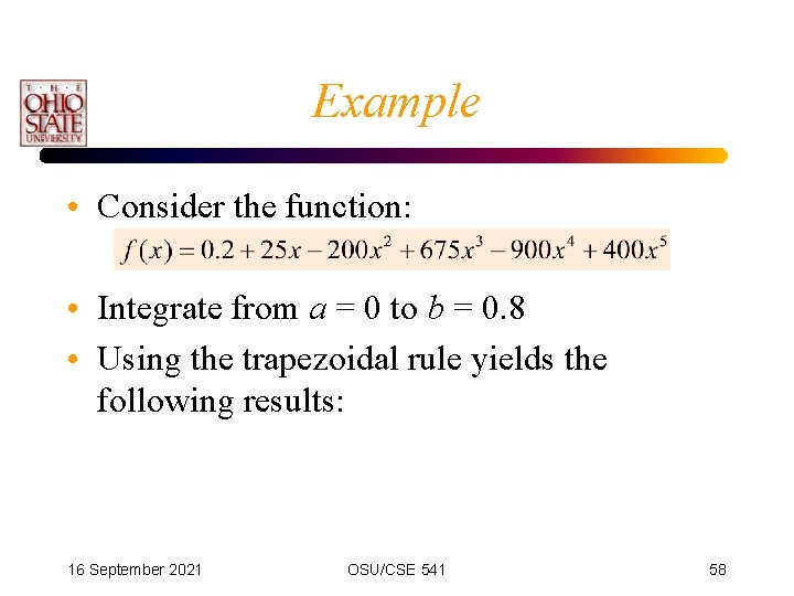
Example • Consider the function: • Integrate from a = 0 to b = 0. 8 • Using the trapezoidal rule yields the following results: 16 September 2021 OSU/CSE 541 58

Example • Trapezoid Rules: k=0 k j k=1 j=0 j=1 j=2 (j=1, k=1) Exact integral is 1. 64053334 16 September 2021 OSU/CSE 541 59

Example k k=0 k=1 j (j=2, k=1) Exact integral is 1. 64053334 16 September 2021 OSU/CSE 541 60

Example k=1 k k=2 j (j=2, k=2) 16 September 2021 OSU/CSE 541 Exact integral is 1. 64053334 61

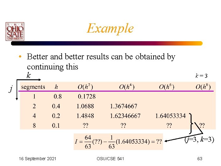
Example k k=1 k=2 k=3 j 16 September 2021 OSU/CSE 541 62

Example • Better and better results can be obtained by continuing this k k=3 j (j=3, k=3) 16 September 2021 OSU/CSE 541 63

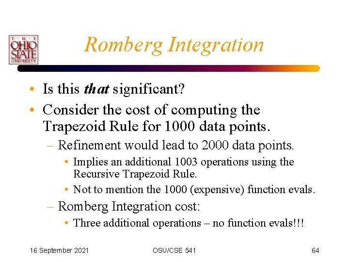
Romberg Integration • Is this that significant? • Consider the cost of computing the Trapezoid Rule for 1000 data points. – Refinement would lead to 2000 data points. • Implies an additional 1003 operations using the Recursive Trapezoid Rule. • Not to mention the 1000 (expensive) function evals. – Romberg Integration cost: • Three additional operations – no function evals!!! 16 September 2021 OSU/CSE 541 64

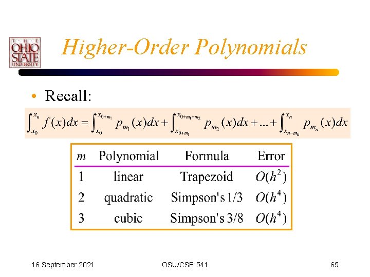
Higher-Order Polynomials • Recall: 16 September 2021 OSU/CSE 541 65

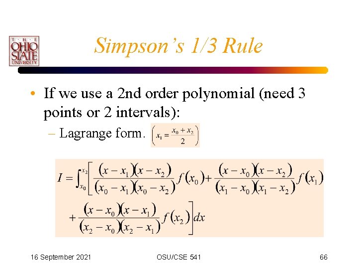
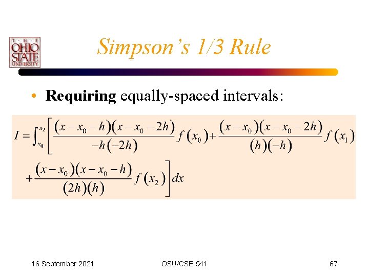
Simpson’s 1/3 Rule • If we use a 2 nd order polynomial (need 3 points or 2 intervals): – Lagrange form. 16 September 2021 OSU/CSE 541 66

Simpson’s 1/3 Rule • Requiring equally-spaced intervals: 16 September 2021 OSU/CSE 541 67

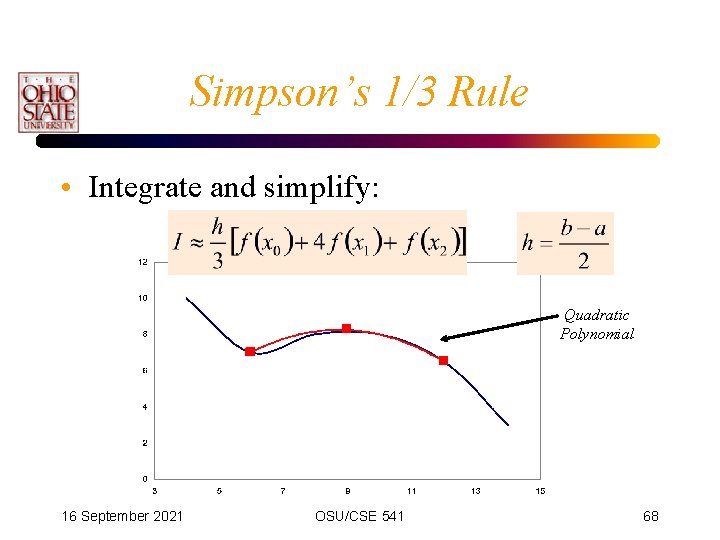
Simpson’s 1/3 Rule • Integrate and simplify: Quadratic Polynomial 16 September 2021 OSU/CSE 541 68

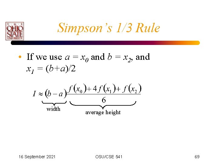
Simpson’s 1/3 Rule • If we use a = x 0 and b = x 2, and x 1 = (b+a)/2 width 16 September 2021 average height OSU/CSE 541 69

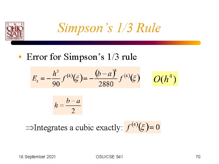
Simpson’s 1/3 Rule • Error for Simpson’s 1/3 rule Integrates a cubic exactly: 16 September 2021 OSU/CSE 541 70

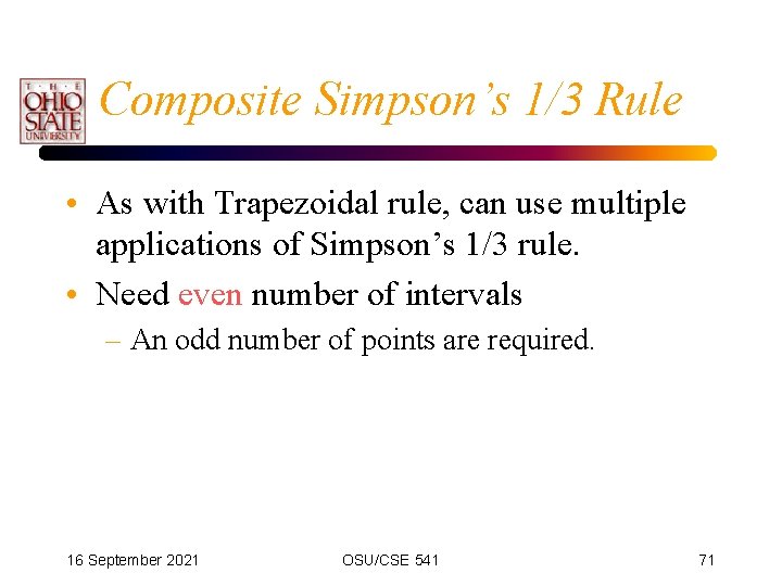
Composite Simpson’s 1/3 Rule • As with Trapezoidal rule, can use multiple applications of Simpson’s 1/3 rule. • Need even number of intervals – An odd number of points are required. 16 September 2021 OSU/CSE 541 71

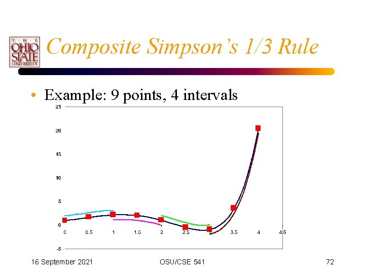
Composite Simpson’s 1/3 Rule • Example: 9 points, 4 intervals 16 September 2021 OSU/CSE 541 72

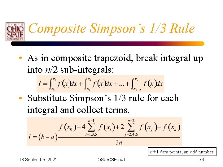
Composite Simpson’s 1/3 Rule • As in composite trapezoid, break integral up into n/2 sub-integrals: • Substitute Simpson’s 1/3 rule for each integral and collect terms. n+1 data points, an odd number 16 September 2021 OSU/CSE 541 73

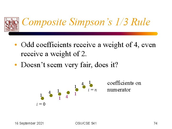
Composite Simpson’s 1/3 Rule • Odd coefficients receive a weight of 4, even receive a weight of 2. • Doesn’t seem very fair, does it? 1 4 1 i=n coefficients on numerator i=0 16 September 2021 OSU/CSE 541 74

Error Estimate • The error can be estimated by: • If n is doubled, h h/2 and Ea Ea/16 is the average 4 th derivative 16 September 2021 OSU/CSE 541 75

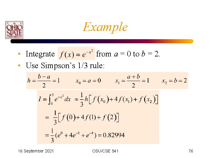
Example • Integrate from a = 0 to b = 2. • Use Simpson’s 1/3 rule: 16 September 2021 OSU/CSE 541 76

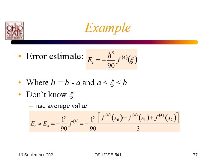
Example • Error estimate: • Where h = b - a and a < < b • Don’t know – use average value 16 September 2021 OSU/CSE 541 77

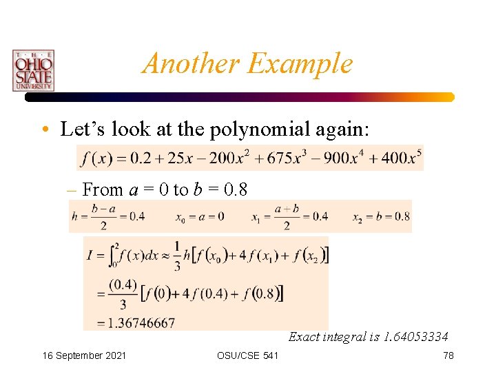
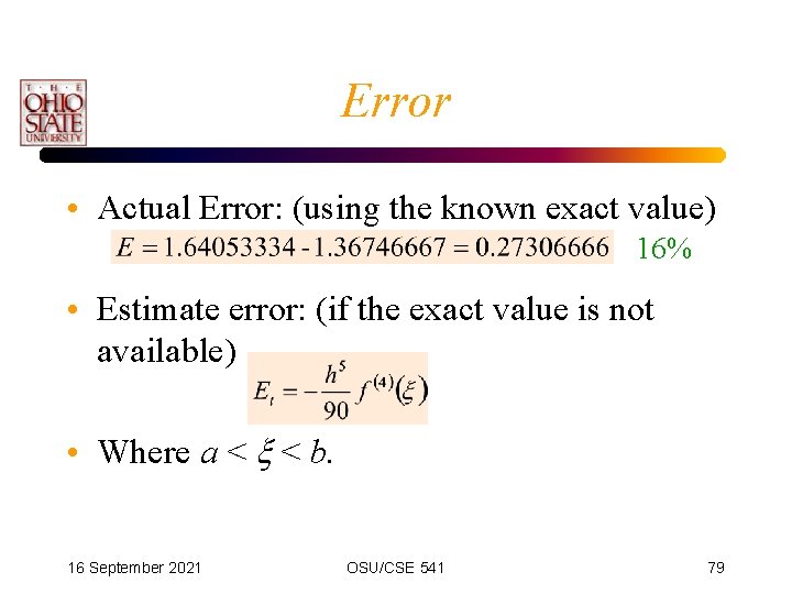
Another Example • Let’s look at the polynomial again: – From a = 0 to b = 0. 8 Exact integral is 1. 64053334 16 September 2021 OSU/CSE 541 78

Error • Actual Error: (using the known exact value) 16% • Estimate error: (if the exact value is not available) • Where a < < b. 16 September 2021 OSU/CSE 541 79

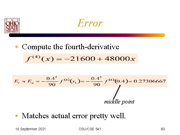
Error • Compute the fourth-derivative middle point • Matches actual error pretty well. 16 September 2021 OSU/CSE 541 80

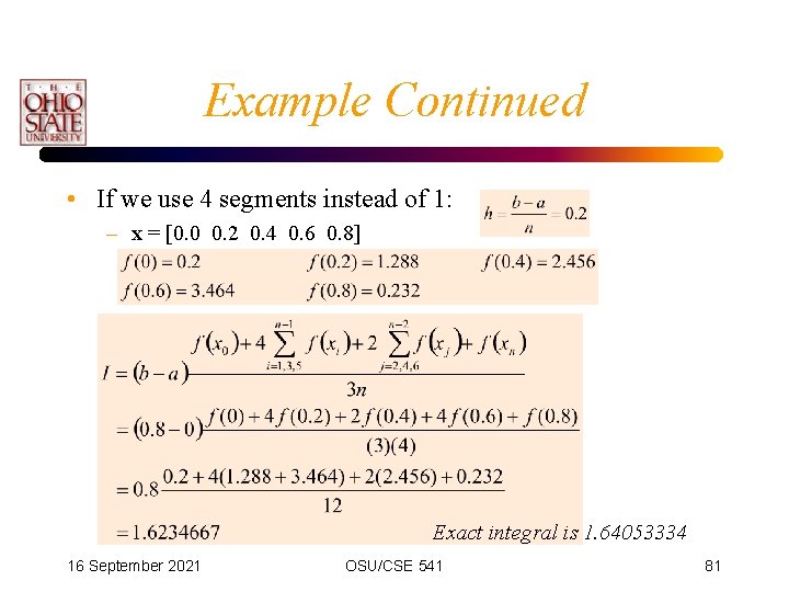
Example Continued • If we use 4 segments instead of 1: – x = [0. 0 0. 2 0. 4 0. 6 0. 8] Exact integral is 1. 64053334 16 September 2021 OSU/CSE 541 81

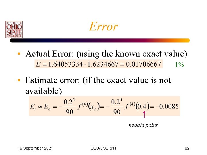
Error • Actual Error: (using the known exact value) 1% • Estimate error: (if the exact value is not available) middle point 16 September 2021 OSU/CSE 541 82

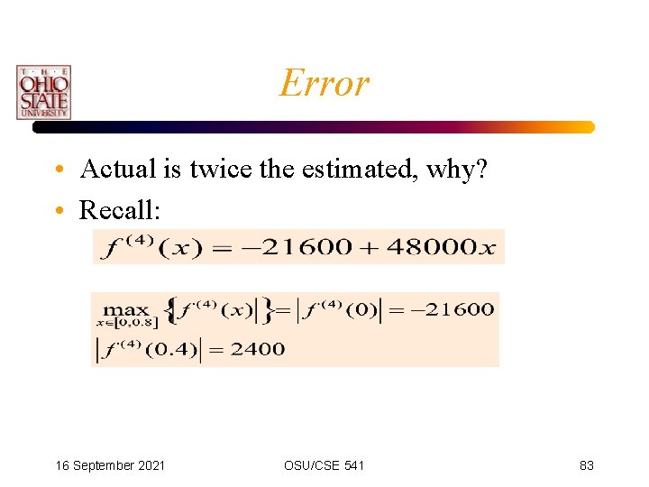
Error • Actual is twice the estimated, why? • Recall: 16 September 2021 OSU/CSE 541 83

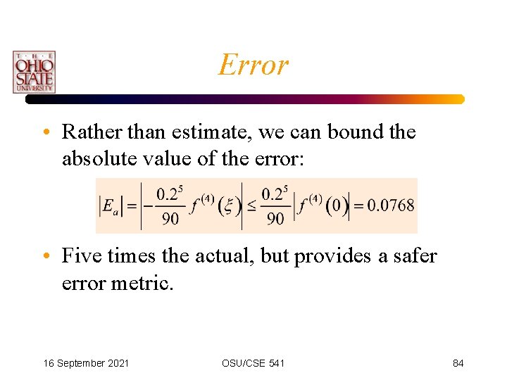
Error • Rather than estimate, we can bound the absolute value of the error: • Five times the actual, but provides a safer error metric. 16 September 2021 OSU/CSE 541 84

Simpon’s 1/3 Rule • Simpson’s 1/3 rule uses a 2 nd order polynomial – need 3 points or 2 intervals – This implies we need an even number of intervals. • What if you don’t have an even number of intervals? Two choices: 1. Use Simpson’s 1/3 on all the segments except the last (or first) one, and use trapezoidal rule on the one left. – Pitfall - larger error on the segment using trapezoid 2. Use Simpson’s 3/8 rule. 16 September 2021 OSU/CSE 541 85

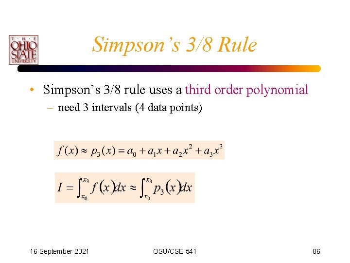
Simpson’s 3/8 Rule • Simpson’s 3/8 rule uses a third order polynomial – need 3 intervals (4 data points) 16 September 2021 OSU/CSE 541 86

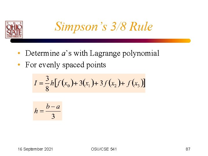
Simpson’s 3/8 Rule • Determine a’s with Lagrange polynomial • For evenly spaced points 16 September 2021 OSU/CSE 541 87

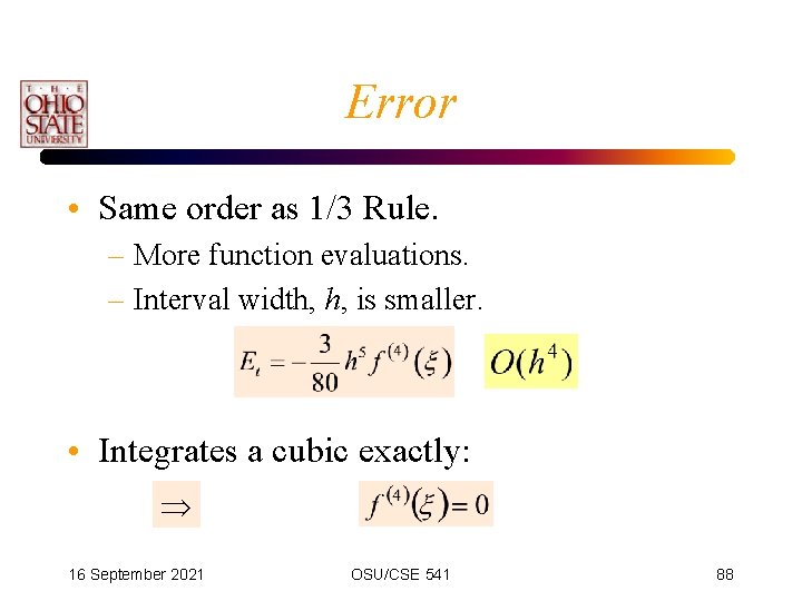
Error • Same order as 1/3 Rule. – More function evaluations. – Interval width, h, is smaller. • Integrates a cubic exactly: 16 September 2021 OSU/CSE 541 88

Comparison • Simpson’s 1/3 rule and Simpson’s 3/8 rule have the same order of error – O(h 4) – trapezoidal rule has an error of O(h 2) • Simpson’s 1/3 rule requires even number of segments. • Simpson’s 3/8 rule requires multiples of three segments. • Both Simpson’s methods require evenly spaced data points 16 September 2021 OSU/CSE 541 89

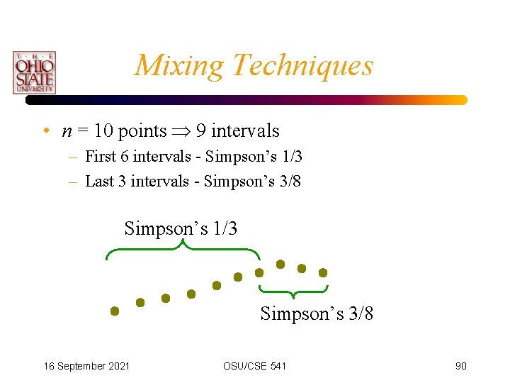
Mixing Techniques • n = 10 points 9 intervals – First 6 intervals - Simpson’s 1/3 – Last 3 intervals - Simpson’s 3/8 Simpson’s 1/3 Simpson’s 3/8 16 September 2021 OSU/CSE 541 90

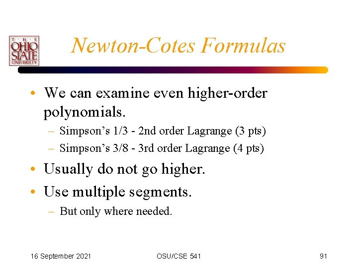
Newton-Cotes Formulas • We can examine even higher-order polynomials. – Simpson’s 1/3 - 2 nd order Lagrange (3 pts) – Simpson’s 3/8 - 3 rd order Lagrange (4 pts) • Usually do not go higher. • Use multiple segments. – But only where needed. 16 September 2021 OSU/CSE 541 91

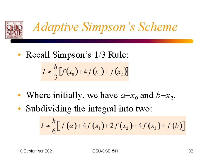
Adaptive Simpson’s Scheme • Recall Simpson’s 1/3 Rule: • Where initially, we have a=x 0 and b=x 2. • Subdividing the integral into two: 16 September 2021 OSU/CSE 541 92

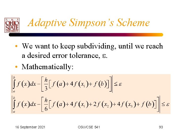
Adaptive Simpson’s Scheme • We want to keep subdividing, until we reach a desired error tolerance, . • Mathematically: 16 September 2021 OSU/CSE 541 93

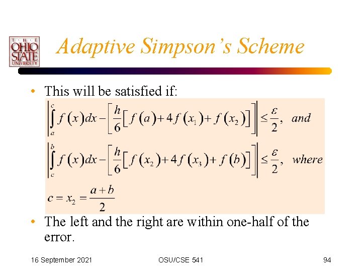
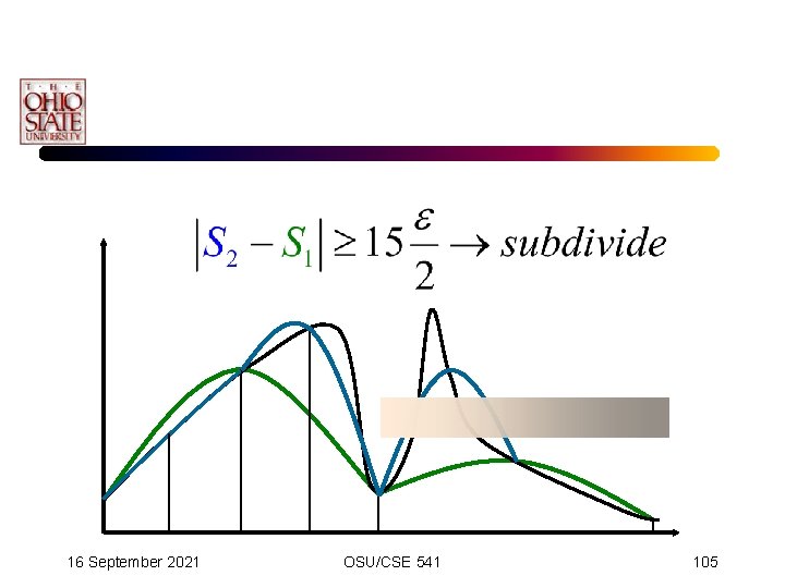
Adaptive Simpson’s Scheme • This will be satisfied if: • The left and the right are within one-half of the error. 16 September 2021 OSU/CSE 541 94

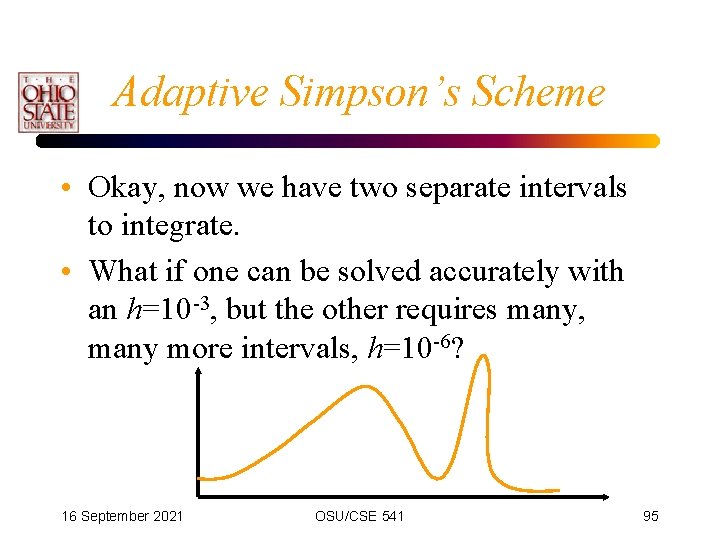
Adaptive Simpson’s Scheme • Okay, now we have two separate intervals to integrate. • What if one can be solved accurately with an h=10 -3, but the other requires many, many more intervals, h=10 -6? 16 September 2021 OSU/CSE 541 95

Adaptive Simpson’s Scheme • Adaptive Simpson’s method provides a divide and conquer scheme until the appropriate error is satisfied everywhere. • Very popular method in practice. • Problem: – We do not know the exact value, and hence do not know the error. 16 September 2021 OSU/CSE 541 96

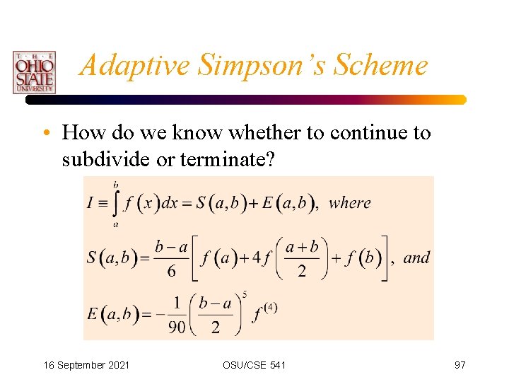
Adaptive Simpson’s Scheme • How do we know whether to continue to subdivide or terminate? 16 September 2021 OSU/CSE 541 97

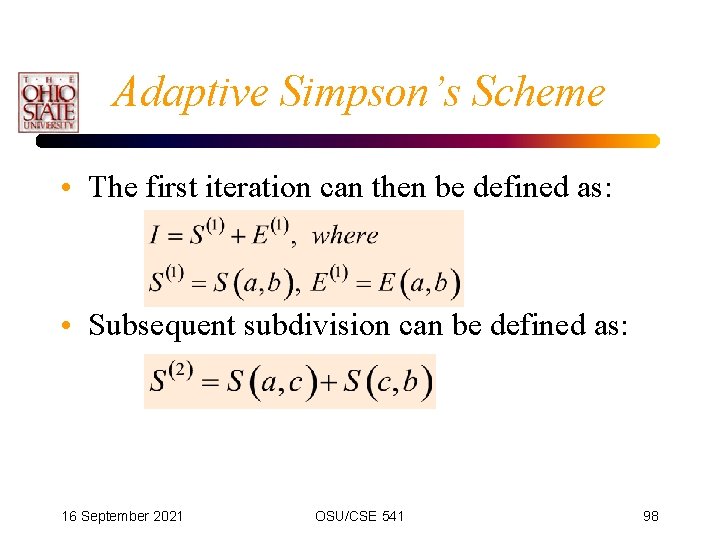
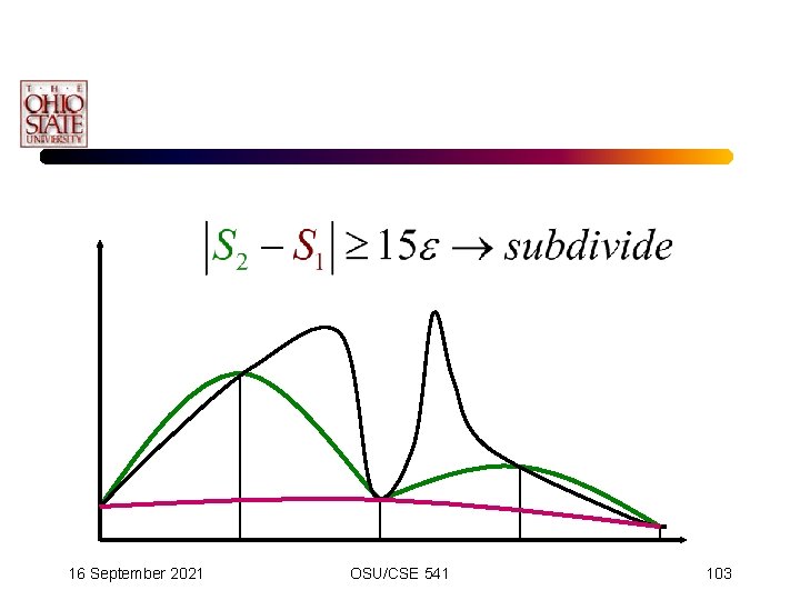
Adaptive Simpson’s Scheme • The first iteration can then be defined as: • Subsequent subdivision can be defined as: 16 September 2021 OSU/CSE 541 98

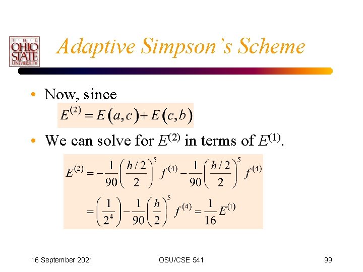
Adaptive Simpson’s Scheme • Now, since • We can solve for E(2) in terms of E(1). 16 September 2021 OSU/CSE 541 99

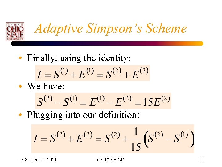
Adaptive Simpson’s Scheme • Finally, using the identity: • We have: • Plugging into our definition: 16 September 2021 OSU/CSE 541 100

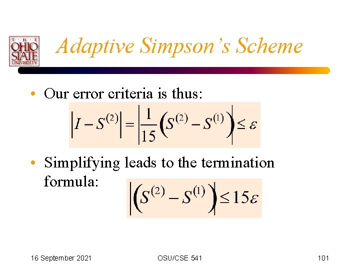
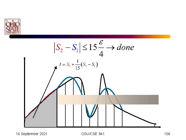
Adaptive Simpson’s Scheme • Our error criteria is thus: • Simplifying leads to the termination formula: 16 September 2021 OSU/CSE 541 101

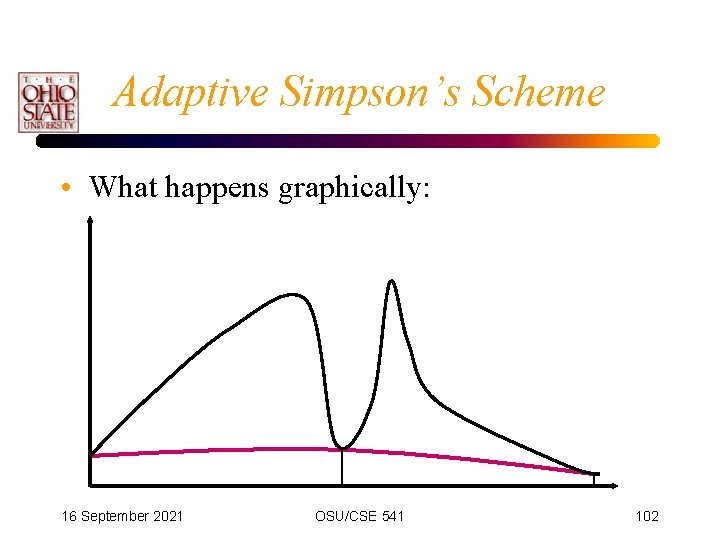
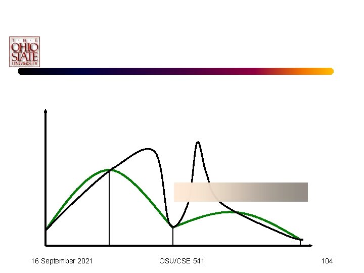
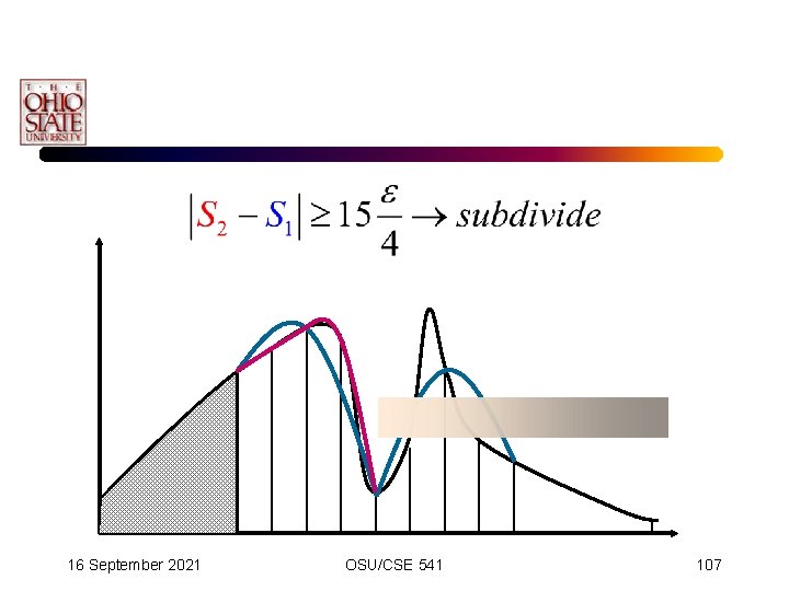
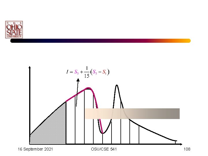
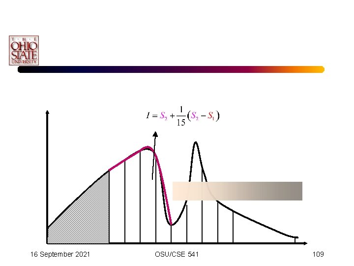
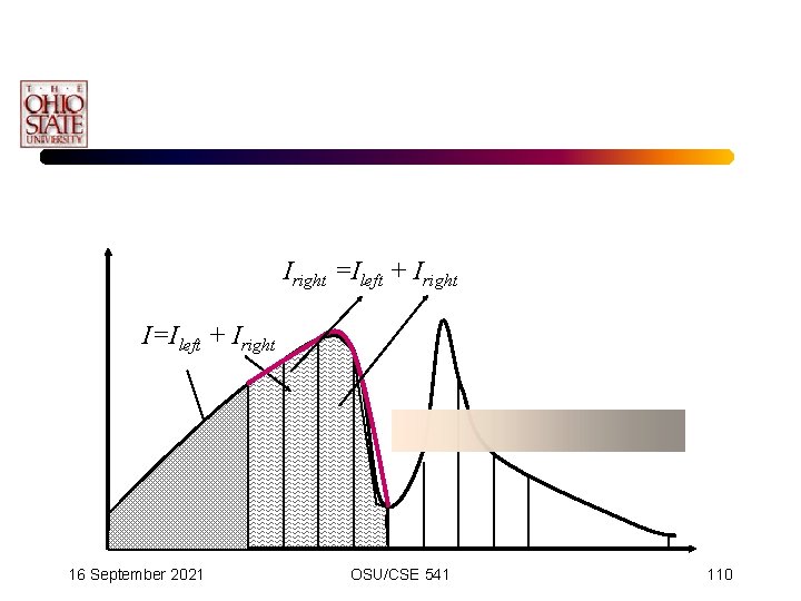
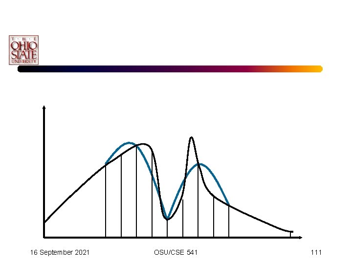
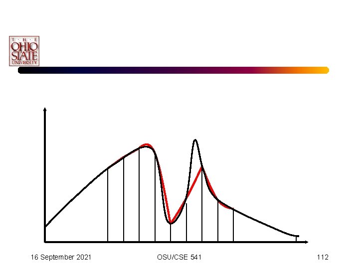
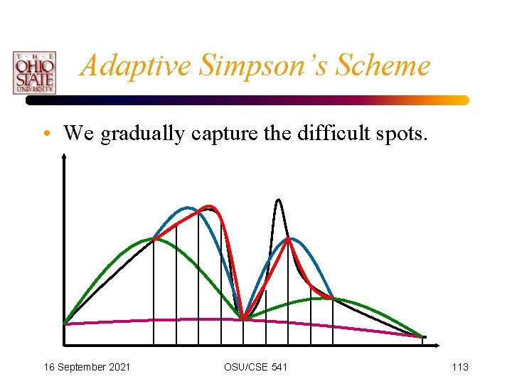
Adaptive Simpson’s Scheme • What happens graphically: 16 September 2021 OSU/CSE 541 102

16 September 2021 OSU/CSE 541 103

16 September 2021 OSU/CSE 541 104

16 September 2021 OSU/CSE 541 105

16 September 2021 OSU/CSE 541 106

16 September 2021 OSU/CSE 541 107

16 September 2021 OSU/CSE 541 108

16 September 2021 OSU/CSE 541 109

Iright =Ileft + Iright I=Ileft + Iright 16 September 2021 OSU/CSE 541 110

16 September 2021 OSU/CSE 541 111

16 September 2021 OSU/CSE 541 112

Adaptive Simpson’s Scheme • We gradually capture the difficult spots. 16 September 2021 OSU/CSE 541 113

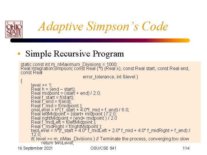
Adaptive Simpson’s Code • Simple Recursive Program static const int m_n. Maximum_Divisions = 1000; Real Integration. Simpson( const Real (*f) (Real x), const Real start, const Real end, const Real error_tolerance, int &level ) { level += 1; Real h = (end – start); Real midpoint = (start + end) / 2. 0; Real f_start = f(start); Real f_end = f(end); Real f_mid = f(midpoint ); one. Level = h*( f_start + 4. 0*f_mid + f_end) / 6. 0; Real left. Midpoint = (start+ midpoint ) / 2. 0; Real right. Midpoint = (end+ midpoint ) / 2. 0 Real f_mid. Left = f(left. Midpoint ); Real f_mid. Right = f(right. Midpoint ); two. Level = h*(f_start + 4. 0* f_mid. Left + 2. 0* f_mid + 4. 0* f_mid. Right + f_end) / 12. 0; if( level >= m_n. Max_Divisions ) // Terminate the process, converging too slow return two. Level; 16 September 2021 OSU/CSE 541 114

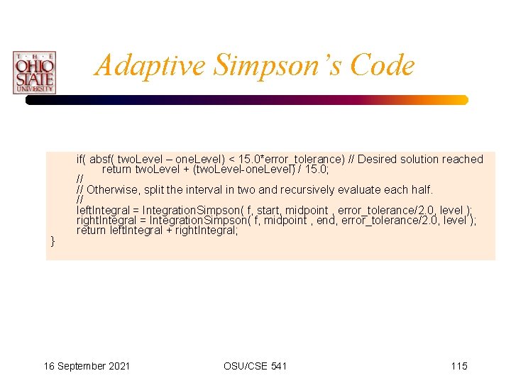
Adaptive Simpson’s Code } if( absf( two. Level – one. Level) < 15. 0*error_tolerance) // Desired solution reached return two. Level + (two. Level-one. Level) / 15. 0; // // Otherwise, split the interval in two and recursively evaluate each half. // left. Integral = Integration. Simpson( f, start, midpoint , error_tolerance/2. 0, level ); right. Integral = Integration. Simpson( f, midpoint , end, error_tolerance/2. 0, level ); return left. Integral + right. Integral; 16 September 2021 OSU/CSE 541 115

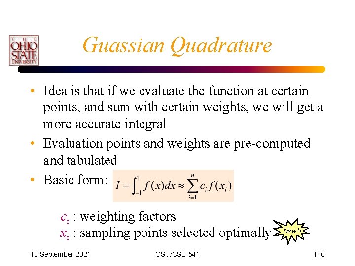
Guassian Quadrature • Idea is that if we evaluate the function at certain points, and sum with certain weights, we will get a more accurate integral • Evaluation points and weights are pre-computed and tabulated • Basic form: ci : weighting factors xi : sampling points selected optimally 16 September 2021 OSU/CSE 541 New!! 116

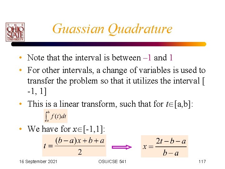
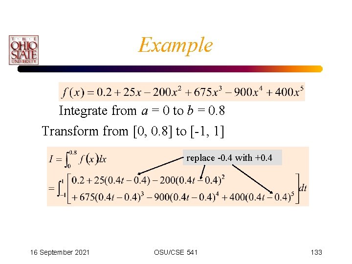
Guassian Quadrature • Note that the interval is between – 1 and 1 • For other intervals, a change of variables is used to transfer the problem so that it utilizes the interval [ -1, 1] • This is a linear transform, such that for t [a, b]: • We have for x [-1, 1]: 16 September 2021 OSU/CSE 541 117

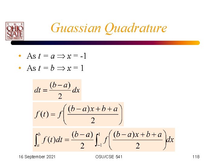
Guassian Quadrature • As t = a x = -1 • As t = b x = 1 16 September 2021 OSU/CSE 541 118

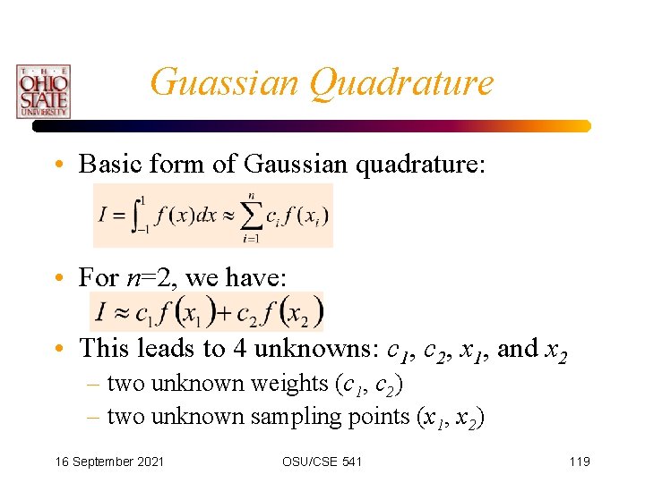
Guassian Quadrature • Basic form of Gaussian quadrature: • For n=2, we have: • This leads to 4 unknowns: c 1, c 2, x 1, and x 2 – two unknown weights (c 1, c 2) – two unknown sampling points (x 1, x 2) 16 September 2021 OSU/CSE 541 119

Guassian Quadrature • What we need now, are four known values for the equation. • If we had these, we could then attempt to solve for the four unknowns. • Let’s make it work for polynomials!!! 16 September 2021 OSU/CSE 541 120

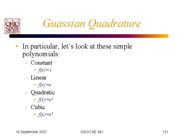
Guassian Quadrature • In particular, let’s look at these simple polynomials: – Constant • f(x)=1 – Linear • f(x)=x – Quadratic • f(x)=x 2 – Cubic • f(x)=x 3 16 September 2021 OSU/CSE 541 121

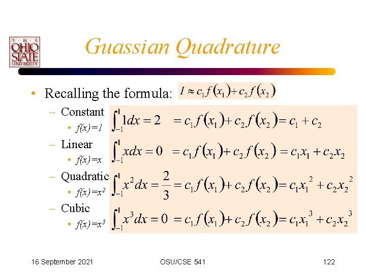
Guassian Quadrature • Recalling the formula: – Constant • f(x)=1 – Linear • f(x)=x – Quadratic • f(x)=x 2 – Cubic • f(x)=x 3 16 September 2021 OSU/CSE 541 122

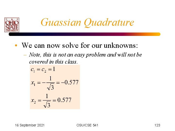
Guassian Quadrature • We can now solve for our unknowns: – Note, this is not an easy problem and will not be covered in this class. 16 September 2021 OSU/CSE 541 123

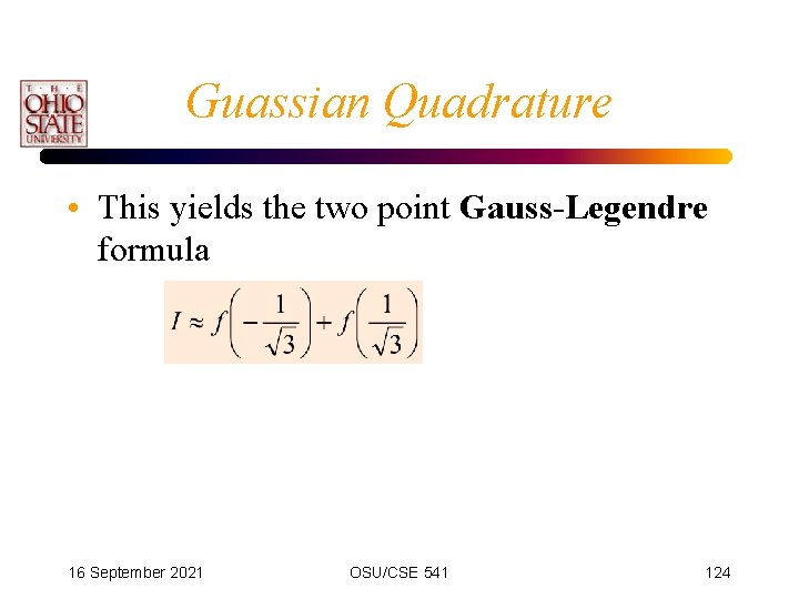
Guassian Quadrature • This yields the two point Gauss-Legendre formula 16 September 2021 OSU/CSE 541 124

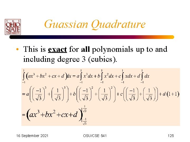
Guassian Quadrature • This is exact for all polynomials up to and including degree 3 (cubics). 16 September 2021 OSU/CSE 541 125

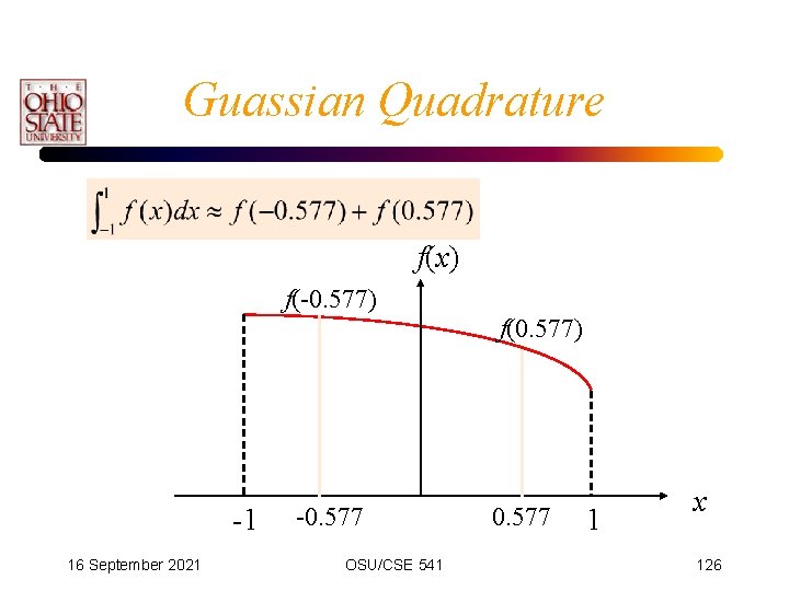
Guassian Quadrature f(x) f(-0. 577) f(0. 577) -1 16 September 2021 -0. 577 OSU/CSE 541 0. 577 1 x 126

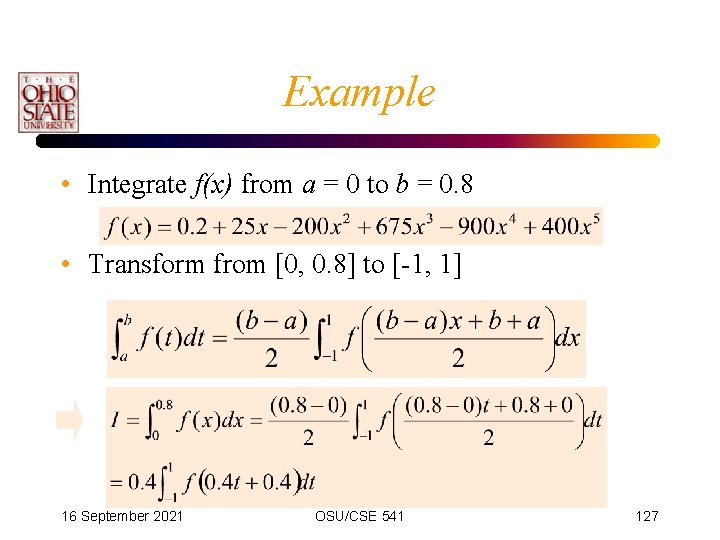
Example • Integrate f(x) from a = 0 to b = 0. 8 • Transform from [0, 0. 8] to [-1, 1] 16 September 2021 OSU/CSE 541 127

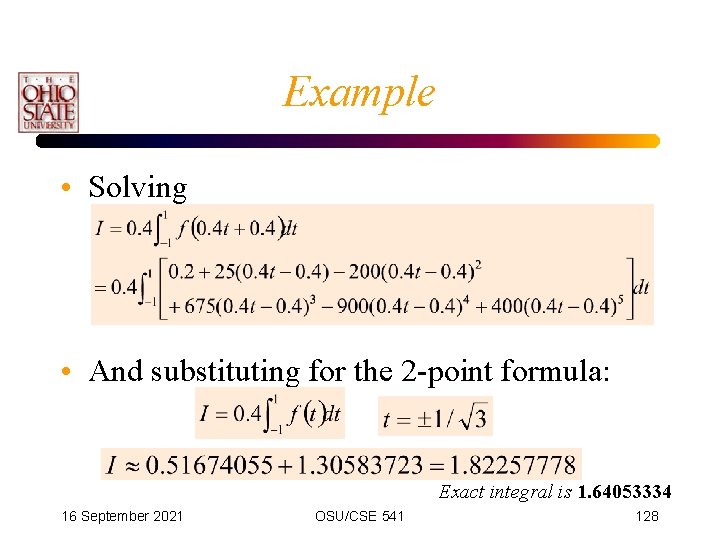
Example • Solving • And substituting for the 2 -point formula: Exact integral is 1. 64053334 16 September 2021 OSU/CSE 541 128

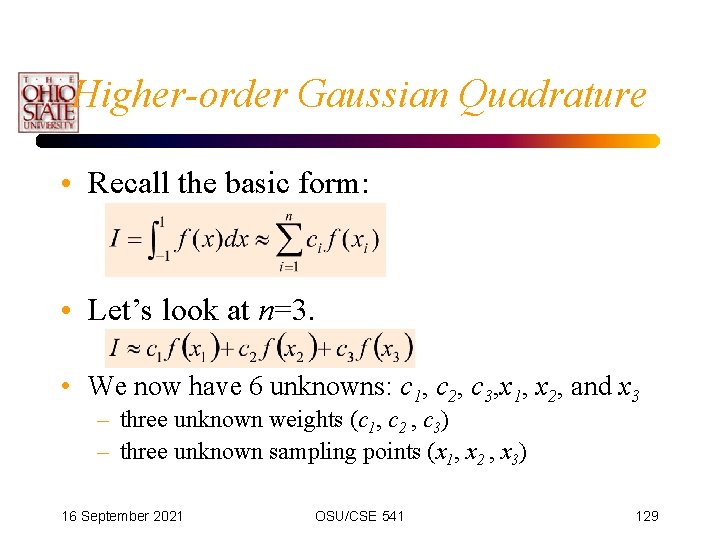
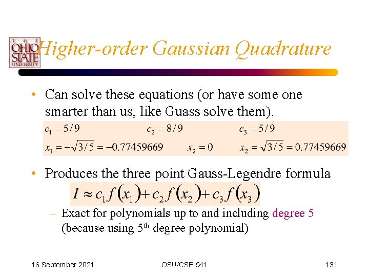
Higher-order Gaussian Quadrature • Recall the basic form: • Let’s look at n=3. • We now have 6 unknowns: c 1, c 2, c 3, x 1, x 2, and x 3 – three unknown weights (c 1, c 2 , c 3) – three unknown sampling points (x 1, x 2 , x 3) 16 September 2021 OSU/CSE 541 129

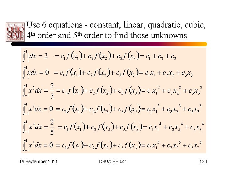
Use 6 equations - constant, linear, quadratic, cubic, 4 th order and 5 th order to find those unknowns 16 September 2021 OSU/CSE 541 130

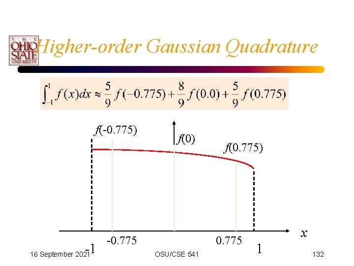
Higher-order Gaussian Quadrature • Can solve these equations (or have some one smarter than us, like Guass solve them). • Produces the three point Gauss-Legendre formula – Exact for polynomials up to and including degree 5 (because using 5 th degree polynomial) 16 September 2021 OSU/CSE 541 131

Higher-order Gaussian Quadrature f(-0. 775) -1 16 September 2021 f(0) -0. 775 f(0. 775) 0. 775 OSU/CSE 541 x 1 132

Example Integrate from a = 0 to b = 0. 8 Transform from [0, 0. 8] to [-1, 1] replace -0. 4 with +0. 4 16 September 2021 OSU/CSE 541 133

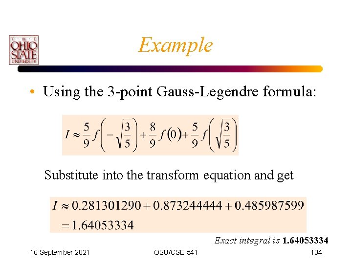
Example • Using the 3 -point Gauss-Legendre formula: Substitute into the transform equation and get Exact integral is 1. 64053334 16 September 2021 OSU/CSE 541 134

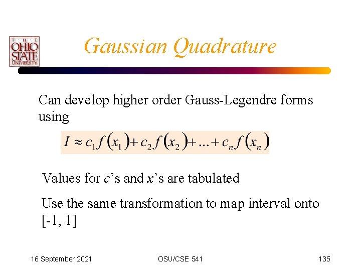
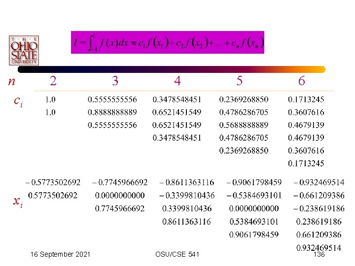
Gaussian Quadrature Can develop higher order Gauss-Legendre forms using Values for c’s and x’s are tabulated Use the same transformation to map interval onto [-1, 1] 16 September 2021 OSU/CSE 541 135

n ci 2 3 4 5 6 xi 16 September 2021 OSU/CSE 541 136

Gaussian Quadrature • Requires function evaluations at nonuniformly spaced points within the integration interval – not appropriate for cases where the function is unknown – not suited for dealing with tabulated data that appear in many engineering problems • If the function is known, its efficiency can be a decided advantage 16 September 2021 OSU/CSE 541 137

Gaussian Quadrature • Problems: – If we add more data points, like doubling the number of sample points. 16 September 2021 OSU/CSE 541 138