Information Theory For Data Management Divesh Srivastava Suresh
![Examples ¨ X uniform over [1, . . . , 4]. H(X) = 2 Examples ¨ X uniform over [1, . . . , 4]. H(X) = 2](https://slidetodoc.com/presentation_image_h/a9df4748910b2d014e3475a7d2f78649/image-13.jpg)
![Conditional Entropy ¨ Let h(x|y) = log 2 1/p(x|y) ¨ H(X|Y) = Ex, y[h(x|y)] Conditional Entropy ¨ Let h(x|y) = log 2 1/p(x|y) ¨ H(X|Y) = Ex, y[h(x|y)]](https://slidetodoc.com/presentation_image_h/a9df4748910b2d014e3475a7d2f78649/image-17.jpg)
![Data Anonymization Using Randomization ¨ X in [0, 10], R 1 = X + Data Anonymization Using Randomization ¨ X in [0, 10], R 1 = X +](https://slidetodoc.com/presentation_image_h/a9df4748910b2d014e3475a7d2f78649/image-24.jpg)
![Data Anonymization Using Randomization ¨ X in [0, 10], R 1 = X + Data Anonymization Using Randomization ¨ X in [0, 10], R 1 = X +](https://slidetodoc.com/presentation_image_h/a9df4748910b2d014e3475a7d2f78649/image-25.jpg)
![Data Anonymization Using Randomization ¨ X in [0, 10], R 1 = X + Data Anonymization Using Randomization ¨ X in [0, 10], R 1 = X +](https://slidetodoc.com/presentation_image_h/a9df4748910b2d014e3475a7d2f78649/image-26.jpg)
![Reconstruction of Original Data Distribution ¨ X in [0, 10], R 1 = X Reconstruction of Original Data Distribution ¨ X in [0, 10], R 1 = X](https://slidetodoc.com/presentation_image_h/a9df4748910b2d014e3475a7d2f78649/image-27.jpg)
![Analysis of Privacy [AS 00] ¨ X in [0, 10], R 1 = X Analysis of Privacy [AS 00] ¨ X in [0, 10], R 1 = X](https://slidetodoc.com/presentation_image_h/a9df4748910b2d014e3475a7d2f78649/image-28.jpg)
![Analysis of Privacy [AA 01] ¨ X in [0, 10], R 1 = X Analysis of Privacy [AA 01] ¨ X in [0, 10], R 1 = X](https://slidetodoc.com/presentation_image_h/a9df4748910b2d014e3475a7d2f78649/image-29.jpg)
![Analysis of Privacy [AA 01] ¨ X in [0, 10], R 1 = X Analysis of Privacy [AA 01] ¨ X in [0, 10], R 1 = X](https://slidetodoc.com/presentation_image_h/a9df4748910b2d014e3475a7d2f78649/image-30.jpg)
![Quantify Loss of Privacy [AA 01] ¨ Goal: quantify loss of privacy based on Quantify Loss of Privacy [AA 01] ¨ Goal: quantify loss of privacy based on](https://slidetodoc.com/presentation_image_h/a9df4748910b2d014e3475a7d2f78649/image-31.jpg)
![Quantify Loss of Privacy [AA 01] ¨ Goal: quantify loss of privacy based on Quantify Loss of Privacy [AA 01] ¨ Goal: quantify loss of privacy based on](https://slidetodoc.com/presentation_image_h/a9df4748910b2d014e3475a7d2f78649/image-32.jpg)
![Quantify Loss of Privacy [AA 01] ¨ Goal: quantify loss of privacy based on Quantify Loss of Privacy [AA 01] ¨ Goal: quantify loss of privacy based on](https://slidetodoc.com/presentation_image_h/a9df4748910b2d014e3475a7d2f78649/image-33.jpg)
![Quantify Loss of Privacy [AA 01] ¨ Goal: quantify loss of privacy based on Quantify Loss of Privacy [AA 01] ¨ Goal: quantify loss of privacy based on](https://slidetodoc.com/presentation_image_h/a9df4748910b2d014e3475a7d2f78649/image-34.jpg)
![Quantify Loss of Privacy [AA 01] ¨ Goal: quantify loss of privacy based on Quantify Loss of Privacy [AA 01] ¨ Goal: quantify loss of privacy based on](https://slidetodoc.com/presentation_image_h/a9df4748910b2d014e3475a7d2f78649/image-35.jpg)
![Quantify Loss of Privacy [AA 01] ¨ Goal: quantify loss of privacy based on Quantify Loss of Privacy [AA 01] ¨ Goal: quantify loss of privacy based on](https://slidetodoc.com/presentation_image_h/a9df4748910b2d014e3475a7d2f78649/image-36.jpg)
![Quantify Loss of Privacy [AA 01] ¨ Equivalent goal: quantify loss of privacy based Quantify Loss of Privacy [AA 01] ¨ Equivalent goal: quantify loss of privacy based](https://slidetodoc.com/presentation_image_h/a9df4748910b2d014e3475a7d2f78649/image-37.jpg)
![Quantify Loss of Privacy ¨ Example: X is uniform in [0, 1] R 3 Quantify Loss of Privacy ¨ Example: X is uniform in [0, 1] R 3](https://slidetodoc.com/presentation_image_h/a9df4748910b2d014e3475a7d2f78649/image-38.jpg)
![Worst Case Loss of Privacy [EGS 03] ¨ Example: X is uniform in [0, Worst Case Loss of Privacy [EGS 03] ¨ Example: X is uniform in [0,](https://slidetodoc.com/presentation_image_h/a9df4748910b2d014e3475a7d2f78649/image-39.jpg)
![Worst Case Loss of Privacy [EGS 03] ¨ Example: X is uniform in [0, Worst Case Loss of Privacy [EGS 03] ¨ Example: X is uniform in [0,](https://slidetodoc.com/presentation_image_h/a9df4748910b2d014e3475a7d2f78649/image-40.jpg)
![Worst Case Loss of Privacy [EGS 03] ¨ Goal: quantify worst case loss of Worst Case Loss of Privacy [EGS 03] ¨ Goal: quantify worst case loss of](https://slidetodoc.com/presentation_image_h/a9df4748910b2d014e3475a7d2f78649/image-41.jpg)
![Worst Case Loss of Privacy [EGS 03] ¨ Example: X is uniform in [0, Worst Case Loss of Privacy [EGS 03] ¨ Example: X is uniform in [0,](https://slidetodoc.com/presentation_image_h/a9df4748910b2d014e3475a7d2f78649/image-42.jpg)
![Worst Case Loss of Privacy [EGS 03] ¨ Example: X is uniform in [5, Worst Case Loss of Privacy [EGS 03] ¨ Example: X is uniform in [5,](https://slidetodoc.com/presentation_image_h/a9df4748910b2d014e3475a7d2f78649/image-43.jpg)
![Information Dependencies [DR 00] ¨ Goal: use information theory to examine and reason about Information Dependencies [DR 00] ¨ Goal: use information theory to examine and reason about](https://slidetodoc.com/presentation_image_h/a9df4748910b2d014e3475a7d2f78649/image-46.jpg)
![Information Dependencies [DR 00] ¨ Functional dependency: X → Y – FD X → Information Dependencies [DR 00] ¨ Functional dependency: X → Y – FD X →](https://slidetodoc.com/presentation_image_h/a9df4748910b2d014e3475a7d2f78649/image-47.jpg)
![Information Dependencies [DR 00] ¨ Functional dependency: X → Y – FD X → Information Dependencies [DR 00] ¨ Functional dependency: X → Y – FD X →](https://slidetodoc.com/presentation_image_h/a9df4748910b2d014e3475a7d2f78649/image-48.jpg)
![Information Dependencies [DR 00] ¨ Result: FD X → Y holds iff H(Y|X) = Information Dependencies [DR 00] ¨ Result: FD X → Y holds iff H(Y|X) =](https://slidetodoc.com/presentation_image_h/a9df4748910b2d014e3475a7d2f78649/image-49.jpg)
![Information Dependencies [DR 00] ¨ Multi-valued dependency: X →→ Y – MVD X →→ Information Dependencies [DR 00] ¨ Multi-valued dependency: X →→ Y – MVD X →→](https://slidetodoc.com/presentation_image_h/a9df4748910b2d014e3475a7d2f78649/image-50.jpg)
![Information Dependencies [DR 00] ¨ Multi-valued dependency: X →→ Y – MVD X →→ Information Dependencies [DR 00] ¨ Multi-valued dependency: X →→ Y – MVD X →→](https://slidetodoc.com/presentation_image_h/a9df4748910b2d014e3475a7d2f78649/image-51.jpg)
![Information Dependencies [DR 00] ¨ Multi-valued dependency: X →→ Y – MVD X →→ Information Dependencies [DR 00] ¨ Multi-valued dependency: X →→ Y – MVD X →→](https://slidetodoc.com/presentation_image_h/a9df4748910b2d014e3475a7d2f78649/image-52.jpg)
![Information Dependencies [DR 00] ¨ Result: MVD X →→ Y holds iff H(Y, Z|X) Information Dependencies [DR 00] ¨ Result: MVD X →→ Y holds iff H(Y, Z|X)](https://slidetodoc.com/presentation_image_h/a9df4748910b2d014e3475a7d2f78649/image-53.jpg)
![Information Dependencies [DR 00] ¨ Result: Armstrong axioms for FDs derivable from In. D Information Dependencies [DR 00] ¨ Result: Armstrong axioms for FDs derivable from In. D](https://slidetodoc.com/presentation_image_h/a9df4748910b2d014e3475a7d2f78649/image-54.jpg)
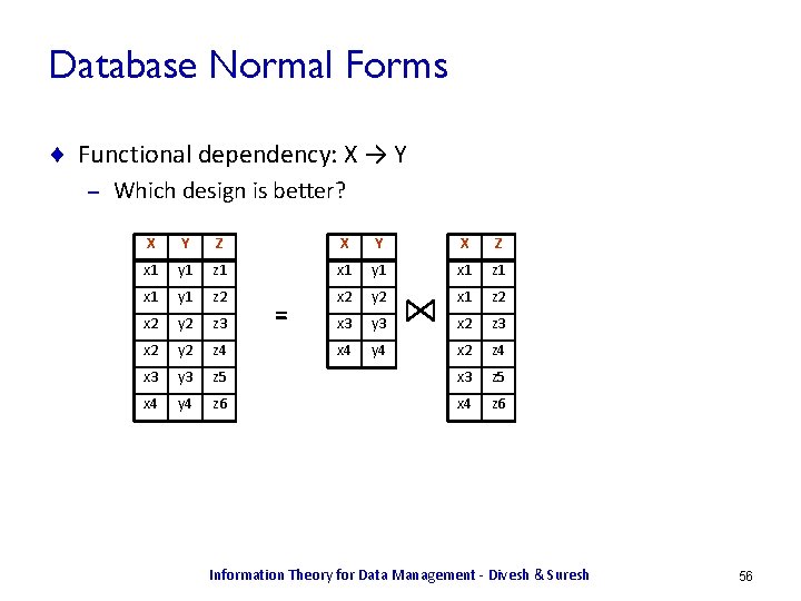
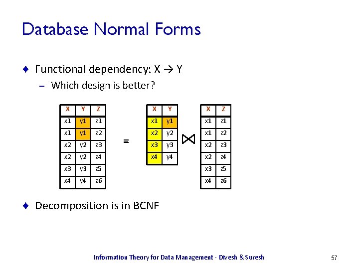
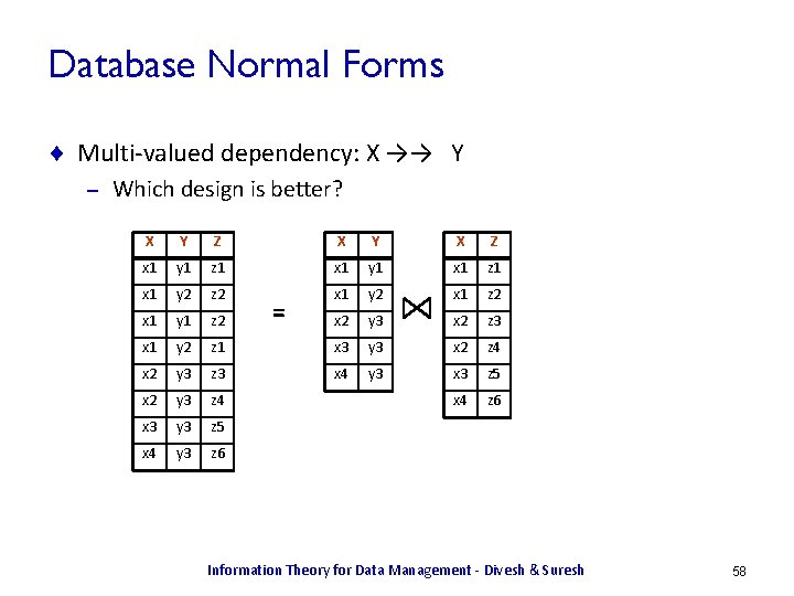
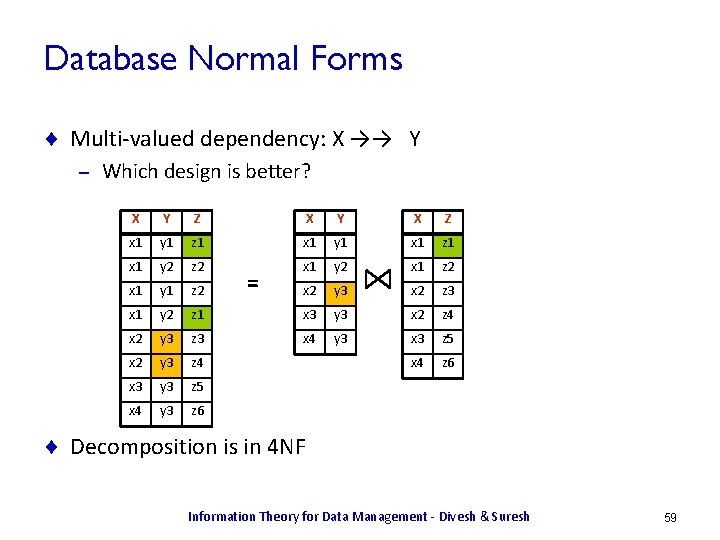
![Well-Designed Databases [AL 03] ¨ Goal: use information theory to characterize “goodness” of a Well-Designed Databases [AL 03] ¨ Goal: use information theory to characterize “goodness” of a](https://slidetodoc.com/presentation_image_h/a9df4748910b2d014e3475a7d2f78649/image-60.jpg)
![Well-Designed Databases [AL 03] ¨ Information content of cell c in database D satisfying Well-Designed Databases [AL 03] ¨ Information content of cell c in database D satisfying](https://slidetodoc.com/presentation_image_h/a9df4748910b2d014e3475a7d2f78649/image-61.jpg)
![Well-Designed Databases [AL 03] ¨ Information content of cell c in database D satisfying Well-Designed Databases [AL 03] ¨ Information content of cell c in database D satisfying](https://slidetodoc.com/presentation_image_h/a9df4748910b2d014e3475a7d2f78649/image-62.jpg)
![Well-Designed Databases [AL 03] ¨ Information content of cell c in database D satisfying Well-Designed Databases [AL 03] ¨ Information content of cell c in database D satisfying](https://slidetodoc.com/presentation_image_h/a9df4748910b2d014e3475a7d2f78649/image-63.jpg)
![Well-Designed Databases [AL 03] ¨ Information content of cell c in database D satisfying Well-Designed Databases [AL 03] ¨ Information content of cell c in database D satisfying](https://slidetodoc.com/presentation_image_h/a9df4748910b2d014e3475a7d2f78649/image-64.jpg)
![Well-Designed Databases [AL 03] ¨ Information content of cell c in database D satisfying Well-Designed Databases [AL 03] ¨ Information content of cell c in database D satisfying](https://slidetodoc.com/presentation_image_h/a9df4748910b2d014e3475a7d2f78649/image-65.jpg)
![Well-Designed Databases [AL 03] ¨ Information content of cell c in DB D satisfying Well-Designed Databases [AL 03] ¨ Information content of cell c in DB D satisfying](https://slidetodoc.com/presentation_image_h/a9df4748910b2d014e3475a7d2f78649/image-66.jpg)
![Well-Designed Databases [AL 03] ¨ Information content of cell c in DB D satisfying Well-Designed Databases [AL 03] ¨ Information content of cell c in DB D satisfying](https://slidetodoc.com/presentation_image_h/a9df4748910b2d014e3475a7d2f78649/image-67.jpg)
![Well-Designed Databases [AL 03] ¨ Information content of cell c in DB D satisfying Well-Designed Databases [AL 03] ¨ Information content of cell c in DB D satisfying](https://slidetodoc.com/presentation_image_h/a9df4748910b2d014e3475a7d2f78649/image-68.jpg)
![Well-Designed Databases [AL 03] ¨ Information content of cell c in DB D satisfying Well-Designed Databases [AL 03] ¨ Information content of cell c in DB D satisfying](https://slidetodoc.com/presentation_image_h/a9df4748910b2d014e3475a7d2f78649/image-69.jpg)
![Well-Designed Databases [AL 03] ¨ Normalization algorithms never decrease information content – Information content Well-Designed Databases [AL 03] ¨ Normalization algorithms never decrease information content – Information content](https://slidetodoc.com/presentation_image_h/a9df4748910b2d014e3475a7d2f78649/image-70.jpg)
![Well-Designed Databases [AL 03] ¨ Normalization algorithms never decrease information content – Information content Well-Designed Databases [AL 03] ¨ Normalization algorithms never decrease information content – Information content](https://slidetodoc.com/presentation_image_h/a9df4748910b2d014e3475a7d2f78649/image-71.jpg)
![Well-Designed Databases [AL 03] ¨ Normalization algorithms never decrease information content – Information content Well-Designed Databases [AL 03] ¨ Normalization algorithms never decrease information content – Information content](https://slidetodoc.com/presentation_image_h/a9df4748910b2d014e3475a7d2f78649/image-72.jpg)
![Opaque Schema Matching [KN 03] ¨ Goal: align columns when column names, data values Opaque Schema Matching [KN 03] ¨ Goal: align columns when column names, data values](https://slidetodoc.com/presentation_image_h/a9df4748910b2d014e3475a7d2f78649/image-83.jpg)
![Opaque Schema Matching [KN 03] ¨ Approach: build complete, labeled graph GD for each Opaque Schema Matching [KN 03] ¨ Approach: build complete, labeled graph GD for each](https://slidetodoc.com/presentation_image_h/a9df4748910b2d014e3475a7d2f78649/image-84.jpg)
![Opaque Schema Matching [KN 03] ¨ Approach: build complete, labeled graph GD for each Opaque Schema Matching [KN 03] ¨ Approach: build complete, labeled graph GD for each](https://slidetodoc.com/presentation_image_h/a9df4748910b2d014e3475a7d2f78649/image-85.jpg)
![Opaque Schema Matching [KN 03] ¨ Approach: build complete, labeled graph GD for each Opaque Schema Matching [KN 03] ¨ Approach: build complete, labeled graph GD for each](https://slidetodoc.com/presentation_image_h/a9df4748910b2d014e3475a7d2f78649/image-86.jpg)
![Opaque Schema Matching [KN 03] ¨ Approach: build complete, labeled graph GD for each Opaque Schema Matching [KN 03] ¨ Approach: build complete, labeled graph GD for each](https://slidetodoc.com/presentation_image_h/a9df4748910b2d014e3475a7d2f78649/image-87.jpg)
![Opaque Schema Matching [KN 03] ¨ Approach: build complete, labeled graph GD for each Opaque Schema Matching [KN 03] ¨ Approach: build complete, labeled graph GD for each](https://slidetodoc.com/presentation_image_h/a9df4748910b2d014e3475a7d2f78649/image-88.jpg)
![Opaque Schema Matching [KN 03] ¨ Approach: build complete, labeled graph GD for each Opaque Schema Matching [KN 03] ¨ Approach: build complete, labeled graph GD for each](https://slidetodoc.com/presentation_image_h/a9df4748910b2d014e3475a7d2f78649/image-89.jpg)
![Opaque Schema Matching [KN 03] ¨ Approach: build complete, labeled graph GD for each Opaque Schema Matching [KN 03] ¨ Approach: build complete, labeled graph GD for each](https://slidetodoc.com/presentation_image_h/a9df4748910b2d014e3475a7d2f78649/image-90.jpg)
![Opaque Schema Matching [KN 03] ¨ Approach: build complete, labeled graph GD for each Opaque Schema Matching [KN 03] ¨ Approach: build complete, labeled graph GD for each](https://slidetodoc.com/presentation_image_h/a9df4748910b2d014e3475a7d2f78649/image-91.jpg)
![Heterogeneity Identification [DKOSV 06] ¨ Goal: identify columns with semantically heterogeneous values – Can Heterogeneity Identification [DKOSV 06] ¨ Goal: identify columns with semantically heterogeneous values – Can](https://slidetodoc.com/presentation_image_h/a9df4748910b2d014e3475a7d2f78649/image-92.jpg)
![Heterogeneity Identification [DKOSV 06] ¨ Example: semantically homogeneous, heterogeneous columns Customer_Id h 8742@yyy. com Heterogeneity Identification [DKOSV 06] ¨ Example: semantically homogeneous, heterogeneous columns Customer_Id h 8742@yyy. com](https://slidetodoc.com/presentation_image_h/a9df4748910b2d014e3475a7d2f78649/image-93.jpg)
![Heterogeneity Identification [DKOSV 06] ¨ Example: semantically homogeneous, heterogeneous columns Customer_Id h 8742@yyy. com Heterogeneity Identification [DKOSV 06] ¨ Example: semantically homogeneous, heterogeneous columns Customer_Id h 8742@yyy. com](https://slidetodoc.com/presentation_image_h/a9df4748910b2d014e3475a7d2f78649/image-94.jpg)
![Heterogeneity Identification [DKOSV 06] ¨ Example: semantically homogeneous, heterogeneous columns Customer_Id h 8742@yyy. com Heterogeneity Identification [DKOSV 06] ¨ Example: semantically homogeneous, heterogeneous columns Customer_Id h 8742@yyy. com](https://slidetodoc.com/presentation_image_h/a9df4748910b2d014e3475a7d2f78649/image-95.jpg)
![Heterogeneity Identification [DKOSV 06] ¨ Example: semantically homogeneous, heterogeneous columns Customer_Id h 8742@yyy. com Heterogeneity Identification [DKOSV 06] ¨ Example: semantically homogeneous, heterogeneous columns Customer_Id h 8742@yyy. com](https://slidetodoc.com/presentation_image_h/a9df4748910b2d014e3475a7d2f78649/image-96.jpg)
![Heterogeneity Identification [DKOSV 06] ¨ Example: semantically homogeneous, heterogeneous columns Customer_Id h 8742@yyy. com Heterogeneity Identification [DKOSV 06] ¨ Example: semantically homogeneous, heterogeneous columns Customer_Id h 8742@yyy. com](https://slidetodoc.com/presentation_image_h/a9df4748910b2d014e3475a7d2f78649/image-97.jpg)
![Heterogeneity Identification [DKOSV 06] ¨ Example: semantically homogeneous, heterogeneous columns Customer_Id 187 -65 -2468 Heterogeneity Identification [DKOSV 06] ¨ Example: semantically homogeneous, heterogeneous columns Customer_Id 187 -65 -2468](https://slidetodoc.com/presentation_image_h/a9df4748910b2d014e3475a7d2f78649/image-98.jpg)
![Heterogeneity Identification [DKOSV 06] ¨ Example: semantically homogeneous, heterogeneous columns Customer_Id 187 -65 -2468 Heterogeneity Identification [DKOSV 06] ¨ Example: semantically homogeneous, heterogeneous columns Customer_Id 187 -65 -2468](https://slidetodoc.com/presentation_image_h/a9df4748910b2d014e3475a7d2f78649/image-99.jpg)
![Heterogeneity Identification [DKOSV 06] ¨ Example: semantically homogeneous, heterogeneous columns Customer_Id 187 -65 -2468 Heterogeneity Identification [DKOSV 06] ¨ Example: semantically homogeneous, heterogeneous columns Customer_Id 187 -65 -2468](https://slidetodoc.com/presentation_image_h/a9df4748910b2d014e3475a7d2f78649/image-100.jpg)
![Heterogeneity Identification [DKOSV 06] ¨ Heterogeneity = complexity of describing the data – – Heterogeneity Identification [DKOSV 06] ¨ Heterogeneity = complexity of describing the data – –](https://slidetodoc.com/presentation_image_h/a9df4748910b2d014e3475a7d2f78649/image-101.jpg)
![Heterogeneity Identification [DKOSV 06] ¨ Hard clustering X = Customer_Id T = Cluster_Id 187 Heterogeneity Identification [DKOSV 06] ¨ Hard clustering X = Customer_Id T = Cluster_Id 187](https://slidetodoc.com/presentation_image_h/a9df4748910b2d014e3475a7d2f78649/image-102.jpg)
![Heterogeneity Identification [DKOSV 06] ¨ Soft clustering: cluster membership probabilities X = Customer_Id T Heterogeneity Identification [DKOSV 06] ¨ Soft clustering: cluster membership probabilities X = Customer_Id T](https://slidetodoc.com/presentation_image_h/a9df4748910b2d014e3475a7d2f78649/image-105.jpg)
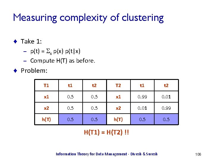
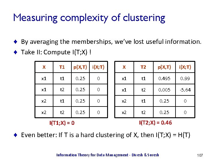
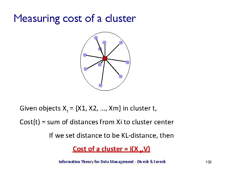
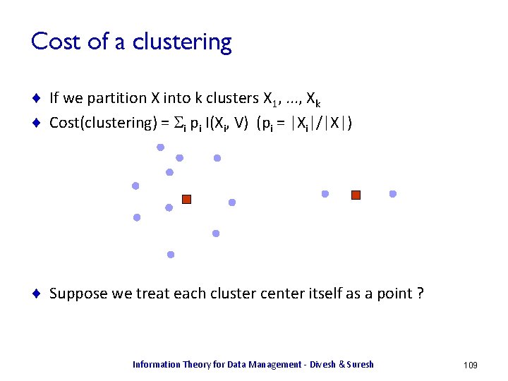
![Heterogeneity Identification [DKOSV 06] ¨ Represent strings as q-gram distributions Customer_Id X = Customer_Id Heterogeneity Identification [DKOSV 06] ¨ Represent strings as q-gram distributions Customer_Id X = Customer_Id](https://slidetodoc.com/presentation_image_h/a9df4748910b2d014e3475a7d2f78649/image-111.jpg)
![Heterogeneity Identification [DKOSV 06] ¨ i. IB: find soft clustering T of X that Heterogeneity Identification [DKOSV 06] ¨ i. IB: find soft clustering T of X that](https://slidetodoc.com/presentation_image_h/a9df4748910b2d014e3475a7d2f78649/image-112.jpg)
![Heterogeneity Identification [DKOSV 06] ¨ Rate distortion curve: I(T; V)/I(X; V) vs I(T; X)/H(X) Heterogeneity Identification [DKOSV 06] ¨ Rate distortion curve: I(T; V)/I(X; V) vs I(T; X)/H(X)](https://slidetodoc.com/presentation_image_h/a9df4748910b2d014e3475a7d2f78649/image-113.jpg)
![Heterogeneity Identification [DKOSV 06] ¨ Heterogeneity = mutual information I(T; X) of i. IB Heterogeneity Identification [DKOSV 06] ¨ Heterogeneity = mutual information I(T; X) of i. IB](https://slidetodoc.com/presentation_image_h/a9df4748910b2d014e3475a7d2f78649/image-114.jpg)
![Heterogeneity Identification [DKOSV 06] ¨ Heterogeneity = mutual information I(T; X) of i. IB Heterogeneity Identification [DKOSV 06] ¨ Heterogeneity = mutual information I(T; X) of i. IB](https://slidetodoc.com/presentation_image_h/a9df4748910b2d014e3475a7d2f78649/image-115.jpg)
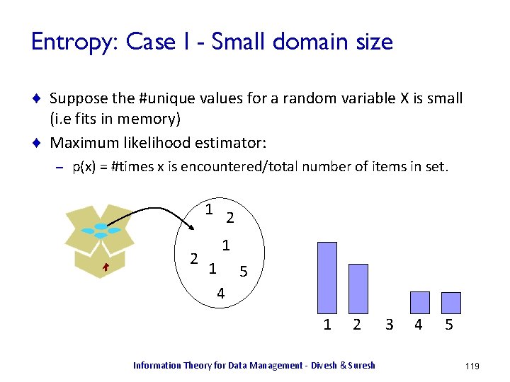
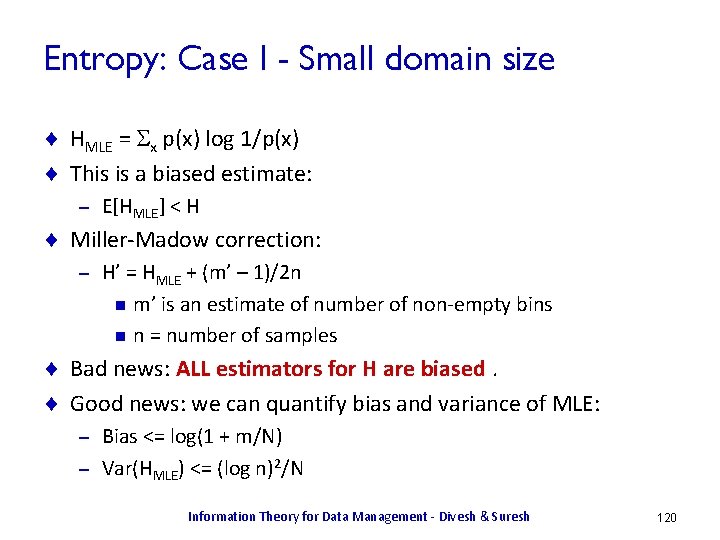
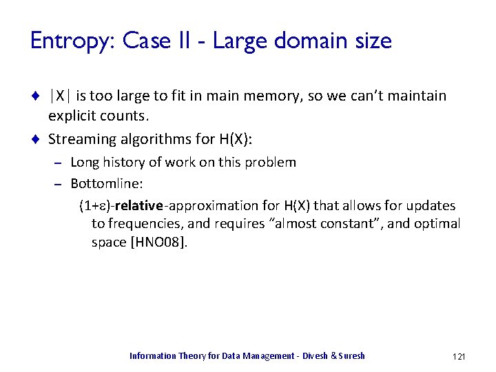
![Streaming Entropy [CCM 07] ¨ High level idea: sample randomly from the stream, and Streaming Entropy [CCM 07] ¨ High level idea: sample randomly from the stream, and](https://slidetodoc.com/presentation_image_h/a9df4748910b2d014e3475a7d2f78649/image-122.jpg)
![Streaming Entropy [CCM 07] ¨ Maintain set of samples from original distribution and distribution Streaming Entropy [CCM 07] ¨ Maintain set of samples from original distribution and distribution](https://slidetodoc.com/presentation_image_h/a9df4748910b2d014e3475a7d2f78649/image-123.jpg)
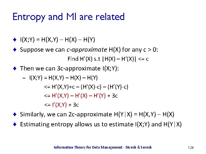
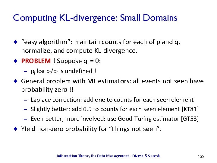
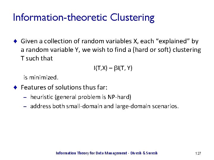
![Agglomerative Clustering (a. IB) [ST 00] ¨ Fix number of clusters k 1. While Agglomerative Clustering (a. IB) [ST 00] ¨ Fix number of clusters k 1. While](https://slidetodoc.com/presentation_image_h/a9df4748910b2d014e3475a7d2f78649/image-128.jpg)
![Agglomerative Clustering (a. IB) [S] ¨ Elegant way of finding the two clusters to Agglomerative Clustering (a. IB) [S] ¨ Elegant way of finding the two clusters to](https://slidetodoc.com/presentation_image_h/a9df4748910b2d014e3475a7d2f78649/image-129.jpg)
![Iterative Information Bottleneck (i. IB) [S] ¨ a. IB yields a hard clustering with Iterative Information Bottleneck (i. IB) [S] ¨ a. IB yields a hard clustering with](https://slidetodoc.com/presentation_image_h/a9df4748910b2d014e3475a7d2f78649/image-130.jpg)
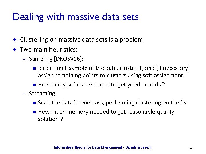
![LIMBO (for a. IB) [ATMS 04] ¨ BIRCH-like idea: Maintain (sparse) summary for each LIMBO (for a. IB) [ATMS 04] ¨ BIRCH-like idea: Maintain (sparse) summary for each](https://slidetodoc.com/presentation_image_h/a9df4748910b2d014e3475a7d2f78649/image-132.jpg)
![References: Information Theory ¨ [CT] Tom Cover and Joy Thomas: Information Theory. ¨ [BMDG References: Information Theory ¨ [CT] Tom Cover and Joy Thomas: Information Theory. ¨ [BMDG](https://slidetodoc.com/presentation_image_h/a9df4748910b2d014e3475a7d2f78649/image-135.jpg)
![References: Data Anonymization ¨ [AA 01] Dakshi Agrawal, Charu C. Aggarwal: On the design References: Data Anonymization ¨ [AA 01] Dakshi Agrawal, Charu C. Aggarwal: On the design](https://slidetodoc.com/presentation_image_h/a9df4748910b2d014e3475a7d2f78649/image-136.jpg)
![References: Database Design ¨ [AL 03] Marcelo Arenas, Leonid Libkin: An information theoretic approach References: Database Design ¨ [AL 03] Marcelo Arenas, Leonid Libkin: An information theoretic approach](https://slidetodoc.com/presentation_image_h/a9df4748910b2d014e3475a7d2f78649/image-137.jpg)
![References: Data Integration ¨ [AMT 04] Periklis Andritsos, Renee J. Miller, Panayiotis Tsaparas: Information-theoretic References: Data Integration ¨ [AMT 04] Periklis Andritsos, Renee J. Miller, Panayiotis Tsaparas: Information-theoretic](https://slidetodoc.com/presentation_image_h/a9df4748910b2d014e3475a7d2f78649/image-138.jpg)
![References: Computing IT quantities ¨ [P 03] Liam Panninski. Estimation of entropy and mutual References: Computing IT quantities ¨ [P 03] Liam Panninski. Estimation of entropy and mutual](https://slidetodoc.com/presentation_image_h/a9df4748910b2d014e3475a7d2f78649/image-139.jpg)
![References: Computing IT quantities ¨ [HNO] Nich Harvey, Jelani Nelson, Krzysztof Onak. Sketching and References: Computing IT quantities ¨ [HNO] Nich Harvey, Jelani Nelson, Krzysztof Onak. Sketching and](https://slidetodoc.com/presentation_image_h/a9df4748910b2d014e3475a7d2f78649/image-140.jpg)
- Slides: 140

Information Theory For Data Management Divesh Srivastava Suresh Venkatasubramanian 1

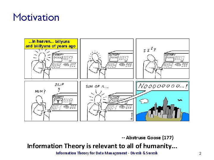
Motivation -- Abstruse Goose (177) Information Theory is relevant to all of humanity. . . Information Theory for Data Management - Divesh & Suresh 2

Background ¨ Many problems in data management need precise reasoning about information content, transfer and loss Structure Extraction – Privacy preservation – Schema design – Probabilistic data ? – Information Theory for Data Management - Divesh & Suresh 3

Information Theory ¨ First developed by Shannon as a way of quantifying capacity of signal channels. ¨ Entropy, relative entropy and mutual information capture intrinsic informational aspects of a signal ¨ Today: Information theory provides a domain-independent way to reason about structure in data – More information = interesting structure – Less information linkage = decoupling of structures – Information Theory for Data Management - Divesh & Suresh 4

Tutorial Thesis Information theory provides a mathematical framework for the quantification of information content, linkage and loss. This framework can be used in the design of data management strategies that rely on probing the structure of information in data. Information Theory for Data Management - Divesh & Suresh 5

Tutorial Goals ¨ ¨ Introduce information-theoretic concepts to DB audience Give a ‘data-centric’ perspective on information theory Connect these to applications in data management Describe underlying computational primitives Illuminate when and how information theory might be of use in new areas of data management. Information Theory for Data Management - Divesh & Suresh 6

Outline Part 1 ¨ Introduction to Information Theory ¨ Application: Data Anonymization ¨ Application: Database Design Part 2 ¨ ¨ Review of Information Theory Basics Application: Data Integration Computing Information Theoretic Primitives Open Problems Information Theory for Data Management - Divesh & Suresh 7

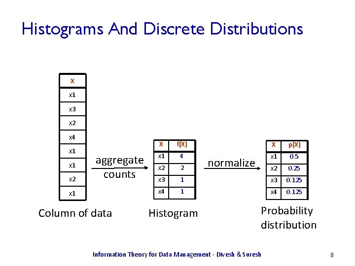
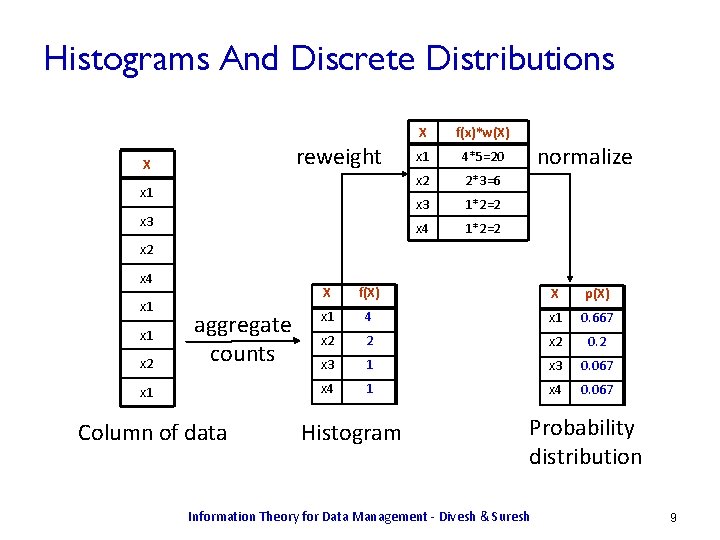
Histograms And Discrete Distributions X x 1 x 3 x 2 x 4 x 1 x 2 aggregate counts x 1 Column of data X f(X) X p(X) x 1 4 x 1 0. 5 x 2 2 x 2 0. 25 x 3 1 x 3 0. 125 x 4 1 x 4 0. 125 Histogram normalize Probability distribution Information Theory for Data Management - Divesh & Suresh 8

Histograms And Discrete Distributions reweight X x 1 x 3 X f(x)*w(X) x 1 4*5=20 x 2 2*3=6 x 3 1*2=2 x 4 1*2=2 normalize x 2 x 4 x 1 x 2 aggregate counts x 1 Column of data X f(X) X p(X) x 1 4 x 1 0. 667 x 2 2 x 2 0. 2 x 3 1 x 3 0. 067 x 4 1 x 4 0. 067 Histogram Probability distribution Information Theory for Data Management - Divesh & Suresh 9

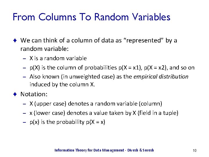
From Columns To Random Variables ¨ We can think of a column of data as “represented” by a random variable: X is a random variable – p(X) is the column of probabilities p(X = x 1), p(X = x 2), and so on – Also known (in unweighted case) as the empirical distribution induced by the column X. – ¨ Notation: X (upper case) denotes a random variable (column) – x (lower case) denotes a value taken by X (field in a tuple) – p(x) is the probability p(X = x) – Information Theory for Data Management - Divesh & Suresh 10

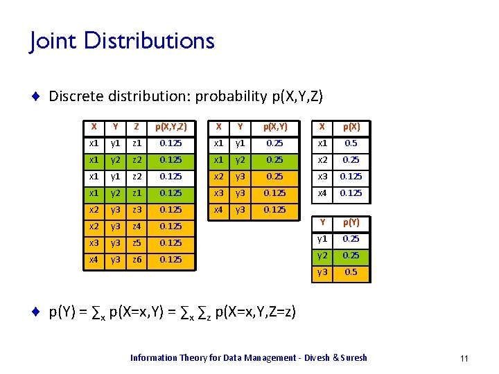
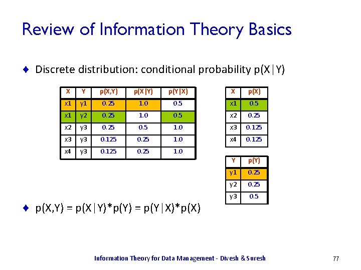
Joint Distributions ¨ Discrete distribution: probability p(X, Y, Z) X Y Z p(X, Y, Z) X Y p(X, Y) X p(X) x 1 y 1 z 1 0. 125 x 1 y 1 0. 25 x 1 0. 5 x 1 y 2 z 2 0. 125 x 1 y 2 0. 25 x 1 y 1 z 2 0. 125 x 2 y 3 0. 25 x 3 0. 125 x 1 y 2 z 1 0. 125 x 3 y 3 0. 125 x 4 0. 125 x 2 y 3 z 3 0. 125 x 4 y 3 0. 125 x 2 y 3 z 4 0. 125 Y p(Y) x 3 y 3 z 5 0. 125 y 1 0. 25 x 4 y 3 z 6 0. 125 y 2 0. 25 y 3 0. 5 ¨ p(Y) = ∑x p(X=x, Y) = ∑x ∑z p(X=x, Y, Z=z) Information Theory for Data Management - Divesh & Suresh 11

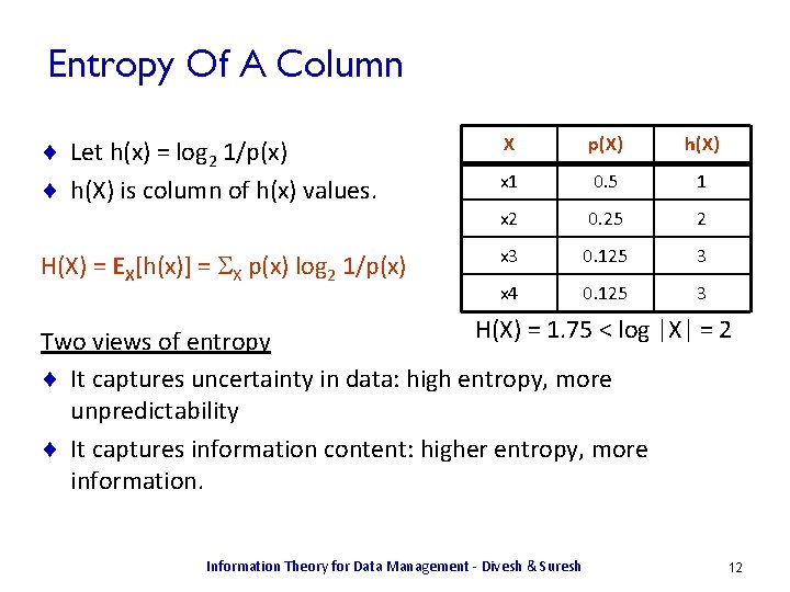
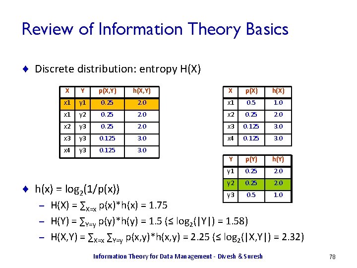
Entropy Of A Column ¨ Let h(x) = log 2 1/p(x) ¨ h(X) is column of h(x) values. H(X) = EX[h(x)] = SX p(x) log 2 1/p(x) X p(X) h(X) x 1 0. 5 1 x 2 0. 25 2 x 3 0. 125 3 x 4 0. 125 3 H(X) = 1. 75 < log |X| = 2 Two views of entropy ¨ It captures uncertainty in data: high entropy, more unpredictability ¨ It captures information content: higher entropy, more information. Information Theory for Data Management - Divesh & Suresh 12
![Examples X uniform over 1 4 HX 2 Examples ¨ X uniform over [1, . . . , 4]. H(X) = 2](https://slidetodoc.com/presentation_image_h/a9df4748910b2d014e3475a7d2f78649/image-13.jpg)
Examples ¨ X uniform over [1, . . . , 4]. H(X) = 2 ¨ Y is 1 with probability 0. 5, in [2, 3, 4] uniformly. H(Y) = 0. 5 log 2 + 0. 5 log 6 ~= 1. 8 < 2 – Y is more sharply defined, and so has less uncertainty. – ¨ Z uniform over [1, . . . , 8]. H(Z) = 3 > 2 – Z spans a larger range, and captures more information X Y Information Theory for Data Management - Divesh & Suresh Z 13

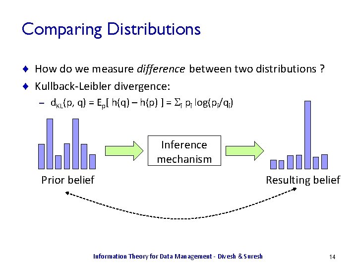
Comparing Distributions ¨ How do we measure difference between two distributions ? ¨ Kullback-Leibler divergence: – d. KL(p, q) = Ep[ h(q) – h(p) ] = Si pi log(pi/qi) Inference mechanism Prior belief Information Theory for Data Management - Divesh & Suresh Resulting belief 14

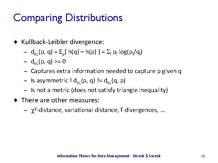
Comparing Distributions ¨ Kullback-Leibler divergence: – – – d. KL(p, q) = Ep[ h(q) – h(p) ] = Si pi log(pi/qi) d. KL(p, q) >= 0 Captures extra information needed to capture p given q Is asymmetric ! d. KL(p, q) != d. KL(q, p) Is not a metric (does not satisfy triangle inequality) ¨ There are other measures: – 2 -distance, variational distance, f-divergences, … Information Theory for Data Management - Divesh & Suresh 15

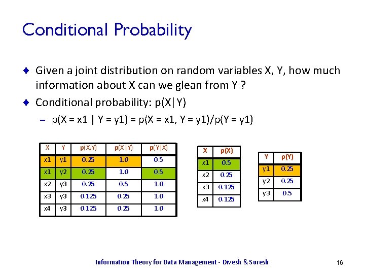
Conditional Probability ¨ Given a joint distribution on random variables X, Y, how much information about X can we glean from Y ? ¨ Conditional probability: p(X|Y) p(X = x 1 | Y = y 1) = p(X = x 1, Y = y 1)/p(Y = y 1) – X Y p(X, Y) p(X|Y) p(Y|X) X p(X) x 1 y 1 0. 25 1. 0 0. 5 x 1 y 2 0. 25 1. 0 0. 5 x 2 0. 25 x 2 y 3 0. 25 0. 5 1. 0 x 3 0. 125 x 3 y 3 0. 125 0. 25 1. 0 x 4 0. 125 x 4 y 3 0. 125 0. 25 1. 0 Y p(Y) y 1 0. 25 y 2 0. 25 y 3 0. 5 Information Theory for Data Management - Divesh & Suresh 16
![Conditional Entropy Let hxy log 2 1pxy HXY Ex yhxy Conditional Entropy ¨ Let h(x|y) = log 2 1/p(x|y) ¨ H(X|Y) = Ex, y[h(x|y)]](https://slidetodoc.com/presentation_image_h/a9df4748910b2d014e3475a7d2f78649/image-17.jpg)
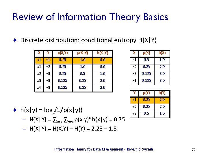
Conditional Entropy ¨ Let h(x|y) = log 2 1/p(x|y) ¨ H(X|Y) = Ex, y[h(x|y)] = Sx Sy p(x, y) log 2 1/p(x|y) ¨ H(X|Y) = H(X, Y) – H(Y) X Y p(X, Y) p(X|Y) h(X|Y) x 1 y 1 0. 25 1. 0 0. 0 x 1 y 2 0. 25 1. 0 0. 0 x 2 y 3 0. 25 0. 5 1. 0 x 3 y 3 0. 125 0. 25 2. 0 x 4 y 3 0. 125 0. 25 2. 0 ¨ H(X|Y) = H(X, Y) – H(Y) = 2. 25 – 1. 5 = 0. 75 ¨ If X, Y are independent, H(X|Y) = H(X) Information Theory for Data Management - Divesh & Suresh 17

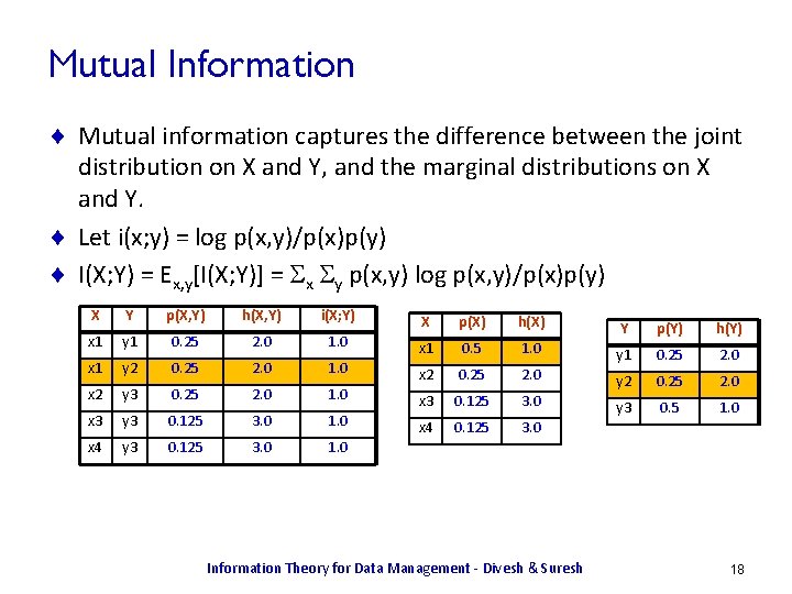
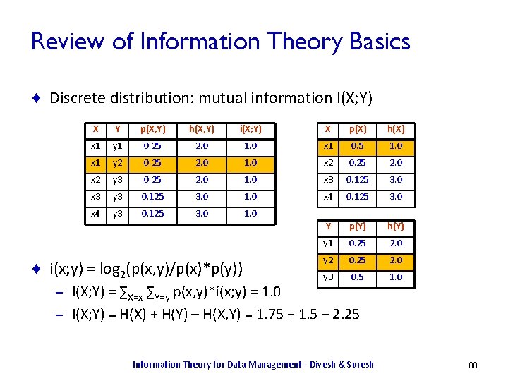
Mutual Information ¨ Mutual information captures the difference between the joint distribution on X and Y, and the marginal distributions on X and Y. ¨ Let i(x; y) = log p(x, y)/p(x)p(y) ¨ I(X; Y) = Ex, y[I(X; Y)] = Sx Sy p(x, y) log p(x, y)/p(x)p(y) X Y p(X, Y) h(X, Y) i(X; Y) X p(X) h(X) x 1 y 1 0. 25 2. 0 1. 0 Y p(Y) h(Y) x 1 0. 5 1. 0 x 1 y 2 0. 25 2. 0 1. 0 y 1 0. 25 2. 0 x 2 y 3 0. 25 2. 0 1. 0 y 2 0. 25 2. 0 x 3 0. 125 3. 0 x 3 y 3 0. 125 3. 0 1. 0 y 3 0. 5 1. 0 x 4 0. 125 3. 0 x 4 y 3 0. 125 3. 0 1. 0 Information Theory for Data Management - Divesh & Suresh 18

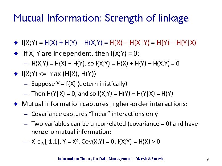
Mutual Information: Strength of linkage ¨ I(X; Y) = H(X) + H(Y) – H(X, Y) = H(X) – H(X|Y) = H(Y) – H(Y|X) ¨ If X, Y are independent, then I(X; Y) = 0: – H(X, Y) = H(X) + H(Y), so I(X; Y) = H(X) + H(Y) – H(X, Y) = 0 ¨ I(X; Y) <= max (H(X), H(Y)) Suppose Y = f(X) (deterministically) – Then H(Y|X) = 0, and so I(X; Y) = H(Y) – H(Y|X) = H(Y) – ¨ Mutual information captures higher-order interactions: Covariance captures “linear” interactions only – Two variables can be uncorrelated (covariance = 0) and have nonzero mutual information: – X R [-1, 1], Y = X 2. Cov(X, Y) = 0, I(X; Y) = H(X) > 0 – Information Theory for Data Management - Divesh & Suresh 19

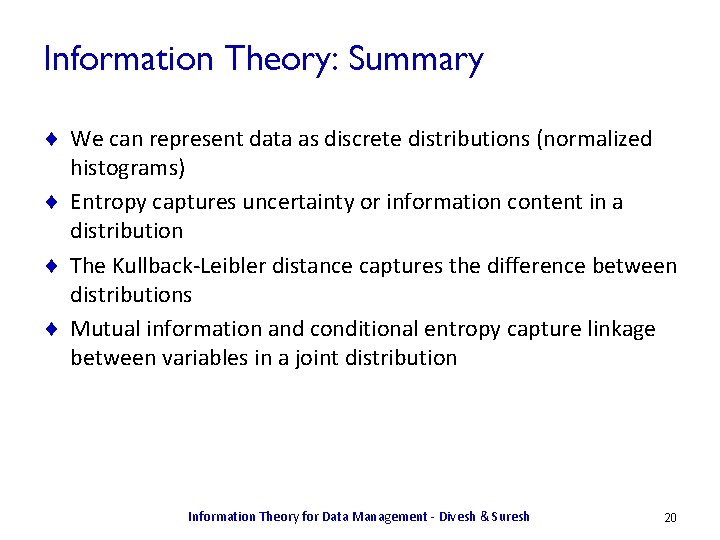
Information Theory: Summary ¨ We can represent data as discrete distributions (normalized histograms) ¨ Entropy captures uncertainty or information content in a distribution ¨ The Kullback-Leibler distance captures the difference between distributions ¨ Mutual information and conditional entropy capture linkage between variables in a joint distribution Information Theory for Data Management - Divesh & Suresh 20

Outline Part 1 ¨ Introduction to Information Theory ¨ Application: Data Anonymization ¨ Application: Database Design Part 2 ¨ ¨ Review of Information Theory Basics Application: Data Integration Computing Information Theoretic Primitives Open Problems Information Theory for Data Management - Divesh & Suresh 21

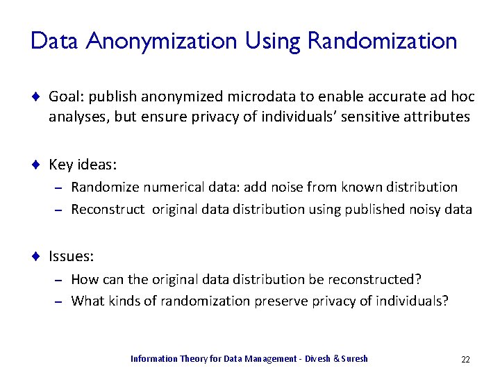
Data Anonymization Using Randomization ¨ Goal: publish anonymized microdata to enable accurate ad hoc analyses, but ensure privacy of individuals’ sensitive attributes ¨ Key ideas: Randomize numerical data: add noise from known distribution – Reconstruct original data distribution using published noisy data – ¨ Issues: How can the original data distribution be reconstructed? – What kinds of randomization preserve privacy of individuals? – Information Theory for Data Management - Divesh & Suresh 22

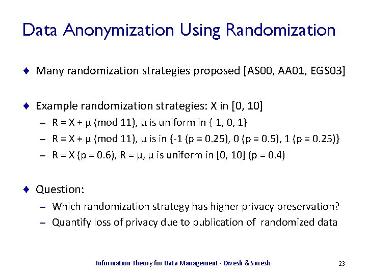
Data Anonymization Using Randomization ¨ Many randomization strategies proposed [AS 00, AA 01, EGS 03] ¨ Example randomization strategies: X in [0, 10] R = X + μ (mod 11), μ is uniform in {-1, 0, 1} – R = X + μ (mod 11), μ is in {-1 (p = 0. 25), 0 (p = 0. 5), 1 (p = 0. 25)} – R = X (p = 0. 6), R = μ, μ is uniform in [0, 10] (p = 0. 4) – ¨ Question: Which randomization strategy has higher privacy preservation? – Quantify loss of privacy due to publication of randomized data – Information Theory for Data Management - Divesh & Suresh 23
![Data Anonymization Using Randomization X in 0 10 R 1 X Data Anonymization Using Randomization ¨ X in [0, 10], R 1 = X +](https://slidetodoc.com/presentation_image_h/a9df4748910b2d014e3475a7d2f78649/image-24.jpg)
Data Anonymization Using Randomization ¨ X in [0, 10], R 1 = X + μ (mod 11), μ is uniform in {-1, 0, 1} Id X s 1 0 s 2 3 s 3 5 s 4 0 s 5 8 s 6 0 s 7 6 s 8 0 Information Theory for Data Management - Divesh & Suresh 24
![Data Anonymization Using Randomization X in 0 10 R 1 X Data Anonymization Using Randomization ¨ X in [0, 10], R 1 = X +](https://slidetodoc.com/presentation_image_h/a9df4748910b2d014e3475a7d2f78649/image-25.jpg)
Data Anonymization Using Randomization ¨ X in [0, 10], R 1 = X + μ (mod 11), μ is uniform in {-1, 0, 1} Id X μ Id R 1 s 1 0 -1 s 1 10 s 2 3 s 3 5 1 s 3 6 s 4 0 0 s 4 0 s 5 8 1 s 5 9 s 6 0 -1 s 6 10 s 7 6 1 s 7 7 s 8 0 0 s 8 0 → Information Theory for Data Management - Divesh & Suresh 25
![Data Anonymization Using Randomization X in 0 10 R 1 X Data Anonymization Using Randomization ¨ X in [0, 10], R 1 = X +](https://slidetodoc.com/presentation_image_h/a9df4748910b2d014e3475a7d2f78649/image-26.jpg)
Data Anonymization Using Randomization ¨ X in [0, 10], R 1 = X + μ (mod 11), μ is uniform in {-1, 0, 1} Id X μ Id R 1 s 1 0 0 s 1 0 s 2 3 -1 s 2 2 s 3 5 0 s 3 5 s 4 0 1 s 4 1 s 5 8 1 s 5 9 s 6 0 -1 s 6 10 s 7 6 -1 s 7 5 s 8 0 1 s 8 1 → Information Theory for Data Management - Divesh & Suresh 26
![Reconstruction of Original Data Distribution X in 0 10 R 1 X Reconstruction of Original Data Distribution ¨ X in [0, 10], R 1 = X](https://slidetodoc.com/presentation_image_h/a9df4748910b2d014e3475a7d2f78649/image-27.jpg)
Reconstruction of Original Data Distribution ¨ X in [0, 10], R 1 = X + μ (mod 11), μ is uniform in {-1, 0, 1} Reconstruct distribution of X using knowledge of R 1 and μ – EM algorithm converges to MLE of original distribution [AA 01] – Id X μ Id R 1 Id X | R 1 s 1 0 0 s 1 {10, 0, 1} s 2 3 -1 s 2 2 s 2 {1, 2, 3} s 3 5 0 s 3 5 s 3 {4, 5, 6} s 4 0 1 s 4 {0, 1, 2} s 5 8 1 s 5 9 s 5 {8, 9, 10} s 6 0 -1 s 6 10 s 6 {9, 10, 0} s 7 6 -1 s 7 5 s 7 {4, 5, 6} s 8 0 1 s 8 {0, 1, 2} → → Information Theory for Data Management - Divesh & Suresh 27
![Analysis of Privacy AS 00 X in 0 10 R 1 X Analysis of Privacy [AS 00] ¨ X in [0, 10], R 1 = X](https://slidetodoc.com/presentation_image_h/a9df4748910b2d014e3475a7d2f78649/image-28.jpg)
Analysis of Privacy [AS 00] ¨ X in [0, 10], R 1 = X + μ (mod 11), μ is uniform in {-1, 0, 1} – If X is uniform in [0, 10], privacy determined by range of μ Id X μ Id R 1 Id X | R 1 s 1 0 0 s 1 {10, 0, 1} s 2 3 -1 s 2 2 s 2 {1, 2, 3} s 3 5 0 s 3 5 s 3 {4, 5, 6} s 4 0 1 s 4 {0, 1, 2} s 5 8 1 s 5 9 s 5 {8, 9, 10} s 6 0 -1 s 6 10 s 6 {9, 10, 0} s 7 6 -1 s 7 5 s 7 {4, 5, 6} s 8 0 1 s 8 {0, 1, 2} → → Information Theory for Data Management - Divesh & Suresh 28
![Analysis of Privacy AA 01 X in 0 10 R 1 X Analysis of Privacy [AA 01] ¨ X in [0, 10], R 1 = X](https://slidetodoc.com/presentation_image_h/a9df4748910b2d014e3475a7d2f78649/image-29.jpg)
Analysis of Privacy [AA 01] ¨ X in [0, 10], R 1 = X + μ (mod 11), μ is uniform in {-1, 0, 1} – If X is uniform in [0, 1] [5, 6], privacy smaller than range of μ Id X μ Id R 1 Id X | R 1 s 1 0 0 s 1 {10, 0, 1} s 2 1 -1 s 2 0 s 2 {10, 0, 1} s 3 5 0 s 3 5 s 3 {4, 5, 6} s 4 6 1 s 4 7 s 4 {6, 7, 8} s 5 0 1 s 5 {0, 1, 2} s 6 1 -1 s 6 0 s 6 {10, 0, 1} s 7 5 -1 s 7 4 s 7 {3, 4, 5} s 8 6 1 s 8 7 s 8 {6, 7, 8} → → Information Theory for Data Management - Divesh & Suresh 29
![Analysis of Privacy AA 01 X in 0 10 R 1 X Analysis of Privacy [AA 01] ¨ X in [0, 10], R 1 = X](https://slidetodoc.com/presentation_image_h/a9df4748910b2d014e3475a7d2f78649/image-30.jpg)
Analysis of Privacy [AA 01] ¨ X in [0, 10], R 1 = X + μ (mod 11), μ is uniform in {-1, 0, 1} If X is uniform in [0, 1] [5, 6], privacy smaller than range of μ – In some cases, sensitive value revealed – Id X μ Id R 1 Id X | R 1 s 1 0 0 s 1 {0, 1} s 2 1 -1 s 2 0 s 2 {0, 1} s 3 5 0 s 3 5 s 3 {5, 6} s 4 6 1 s 4 7 s 4 {6} s 5 0 1 s 5 {0, 1} s 6 1 -1 s 6 0 s 6 {0, 1} s 7 5 -1 s 7 4 s 7 {5} s 8 6 1 s 8 7 s 8 {6} → → Information Theory for Data Management - Divesh & Suresh 30
![Quantify Loss of Privacy AA 01 Goal quantify loss of privacy based on Quantify Loss of Privacy [AA 01] ¨ Goal: quantify loss of privacy based on](https://slidetodoc.com/presentation_image_h/a9df4748910b2d014e3475a7d2f78649/image-31.jpg)
Quantify Loss of Privacy [AA 01] ¨ Goal: quantify loss of privacy based on mutual information I(X; R) Smaller H(X|R) more loss of privacy in X by knowledge of R – Larger I(X; R) more loss of privacy in X by knowledge of R – I(X; R) = H(X) – H(X|R) – ¨ I(X; R) used to capture correlation between X and R p(X) is the prior knowledge of sensitive attribute X – p(X, R) is the joint distribution of X and R – Information Theory for Data Management - Divesh & Suresh 31
![Quantify Loss of Privacy AA 01 Goal quantify loss of privacy based on Quantify Loss of Privacy [AA 01] ¨ Goal: quantify loss of privacy based on](https://slidetodoc.com/presentation_image_h/a9df4748910b2d014e3475a7d2f78649/image-32.jpg)
Quantify Loss of Privacy [AA 01] ¨ Goal: quantify loss of privacy based on mutual information I(X; R) – X is uniform in [5, 6], R 1 = X + μ (mod 11), μ is uniform in {-1, 0, 1} X R 1 p(X, R 1) h(X, R 1) i(X; R 1) X 5 4 5 5 5 6 6 5 R 1 6 6 4 6 7 5 p(X) h(X) p(R 1) h(R 1) 6 7 Information Theory for Data Management - Divesh & Suresh 32
![Quantify Loss of Privacy AA 01 Goal quantify loss of privacy based on Quantify Loss of Privacy [AA 01] ¨ Goal: quantify loss of privacy based on](https://slidetodoc.com/presentation_image_h/a9df4748910b2d014e3475a7d2f78649/image-33.jpg)
Quantify Loss of Privacy [AA 01] ¨ Goal: quantify loss of privacy based on mutual information I(X; R) – X is uniform in [5, 6], R 1 = X + μ (mod 11), μ is uniform in {-1, 0, 1} X R 1 p(X, R 1) h(X, R 1) i(X; R 1) X p(X) 5 4 0. 17 5 0. 5 5 5 0. 17 6 0. 5 5 6 0. 17 6 5 0. 17 R 1 p(R 1) 6 6 0. 17 4 0. 17 6 7 0. 17 5 0. 34 6 0. 34 7 0. 17 h(X) h(R 1) Information Theory for Data Management - Divesh & Suresh 33
![Quantify Loss of Privacy AA 01 Goal quantify loss of privacy based on Quantify Loss of Privacy [AA 01] ¨ Goal: quantify loss of privacy based on](https://slidetodoc.com/presentation_image_h/a9df4748910b2d014e3475a7d2f78649/image-34.jpg)
Quantify Loss of Privacy [AA 01] ¨ Goal: quantify loss of privacy based on mutual information I(X; R) – X is uniform in [5, 6], R 1 = X + μ (mod 11), μ is uniform in {-1, 0, 1} X R 1 p(X, R 1) h(X, R 1) i(X; R 1) X p(X) h(X) 5 4 0. 17 2. 58 5 0. 5 1. 0 5 5 0. 17 2. 58 6 0. 5 1. 0 5 6 0. 17 2. 58 6 5 0. 17 2. 58 R 1 p(R 1) h(R 1) 6 6 0. 17 2. 58 4 0. 17 2. 58 6 7 0. 17 2. 58 5 0. 34 1. 58 6 0. 34 1. 58 7 0. 17 2. 58 Information Theory for Data Management - Divesh & Suresh 34
![Quantify Loss of Privacy AA 01 Goal quantify loss of privacy based on Quantify Loss of Privacy [AA 01] ¨ Goal: quantify loss of privacy based on](https://slidetodoc.com/presentation_image_h/a9df4748910b2d014e3475a7d2f78649/image-35.jpg)
Quantify Loss of Privacy [AA 01] ¨ Goal: quantify loss of privacy based on mutual information I(X; R) X is uniform in [5, 6], R 1 = X + μ (mod 11), μ is uniform in {-1, 0, 1} – I(X; R) = 0. 33 – X R 1 p(X, R 1) h(X, R 1) i(X; R 1) X p(X) h(X) 5 4 0. 17 2. 58 1. 0 5 0. 5 1. 0 5 5 0. 17 2. 58 0. 0 6 0. 5 1. 0 5 6 0. 17 2. 58 0. 0 6 5 0. 17 2. 58 0. 0 R 1 p(R 1) h(R 1) 6 6 0. 17 2. 58 0. 0 4 0. 17 2. 58 6 7 0. 17 2. 58 1. 0 5 0. 34 1. 58 6 0. 34 1. 58 7 0. 17 2. 58 Information Theory for Data Management - Divesh & Suresh 35
![Quantify Loss of Privacy AA 01 Goal quantify loss of privacy based on Quantify Loss of Privacy [AA 01] ¨ Goal: quantify loss of privacy based on](https://slidetodoc.com/presentation_image_h/a9df4748910b2d014e3475a7d2f78649/image-36.jpg)
Quantify Loss of Privacy [AA 01] ¨ Goal: quantify loss of privacy based on mutual information I(X; R) X is uniform in [5, 6], R 2 = X + μ (mod 11), μ is uniform in {0, 1} – I(X; R 1) = 0. 33, I(X; R 2) = 0. 5 R 2 is a bigger privacy risk than R 1 – X R 2 p(X, R 2) h(X, R 2) i(X; R 2) X p(X) h(X) 5 5 0. 25 2. 0 1. 0 5 0. 5 1. 0 5 6 0. 25 2. 0 0. 0 6 0. 5 1. 0 6 6 0. 25 2. 0 0. 0 6 7 0. 25 2. 0 1. 0 R 2 p(R 2) h(R 2) 5 0. 25 2. 0 6 0. 5 1. 0 7 0. 25 2. 0 Information Theory for Data Management - Divesh & Suresh 36
![Quantify Loss of Privacy AA 01 Equivalent goal quantify loss of privacy based Quantify Loss of Privacy [AA 01] ¨ Equivalent goal: quantify loss of privacy based](https://slidetodoc.com/presentation_image_h/a9df4748910b2d014e3475a7d2f78649/image-37.jpg)
Quantify Loss of Privacy [AA 01] ¨ Equivalent goal: quantify loss of privacy based on H(X|R) X is uniform in [5, 6], R 2 = X + μ (mod 11), μ is uniform in {0, 1} – Intuition: we know more about X given R 2, than about X given R 1 – H(X|R 1) = 0. 67, H(X|R 2) = 0. 5 R 2 is a bigger privacy risk than R 1 – X R 1 p(X, R 1) p(X|R 1) h(X|R 1) X R 2 p(X, R 2) p(X|R 2) h(X|R 2) 5 4 0. 17 1. 0 0. 0 5 5 0. 25 1. 0 0. 0 5 5 0. 17 0. 5 1. 0 5 6 0. 25 0. 5 1. 0 5 6 0. 17 0. 5 1. 0 6 6 0. 25 0. 5 1. 0 6 5 0. 17 0. 5 1. 0 6 7 0. 25 1. 0 0. 0 6 6 0. 17 0. 5 1. 0 6 7 0. 17 1. 0 0. 0 Information Theory for Data Management - Divesh & Suresh 37
![Quantify Loss of Privacy Example X is uniform in 0 1 R 3 Quantify Loss of Privacy ¨ Example: X is uniform in [0, 1] R 3](https://slidetodoc.com/presentation_image_h/a9df4748910b2d014e3475a7d2f78649/image-38.jpg)
Quantify Loss of Privacy ¨ Example: X is uniform in [0, 1] R 3 = e (p = 0. 9999), R 3 = X (p = 0. 0001) – R 4 = X (p = 0. 6), R 4 = 1 – X (p = 0. 4) – ¨ Is R 3 or R 4 a bigger privacy risk? Information Theory for Data Management - Divesh & Suresh 38
![Worst Case Loss of Privacy EGS 03 Example X is uniform in 0 Worst Case Loss of Privacy [EGS 03] ¨ Example: X is uniform in [0,](https://slidetodoc.com/presentation_image_h/a9df4748910b2d014e3475a7d2f78649/image-39.jpg)
Worst Case Loss of Privacy [EGS 03] ¨ Example: X is uniform in [0, 1] R 3 = e (p = 0. 9999), R 3 = X (p = 0. 0001) – R 4 = X (p = 0. 6), R 4 = 1 – X (p = 0. 4) – X R 3 p(X, R 3) h(X, R 3) i(X; R 3) X R 4 p(X, R 4) h(X, R 4) i(X; R 4) 0 e 0. 49995 1. 0 0 0 0. 3 1. 74 0. 26 0 0 0. 00005 14. 29 1. 0 0 1 0. 2 2. 32 -0. 32 1 e 0. 49995 1. 0 0. 0 1 0 0. 2 2. 32 -0. 32 1 1 0. 00005 14. 29 1. 0 1 1 0. 3 1. 74 0. 26 ¨ I(X; R 3) = 0. 0001 << I(X; R 4) = 0. 028 Information Theory for Data Management - Divesh & Suresh 39
![Worst Case Loss of Privacy EGS 03 Example X is uniform in 0 Worst Case Loss of Privacy [EGS 03] ¨ Example: X is uniform in [0,](https://slidetodoc.com/presentation_image_h/a9df4748910b2d014e3475a7d2f78649/image-40.jpg)
Worst Case Loss of Privacy [EGS 03] ¨ Example: X is uniform in [0, 1] R 3 = e (p = 0. 9999), R 3 = X (p = 0. 0001) – R 4 = X (p = 0. 6), R 4 = 1 – X (p = 0. 4) – X R 3 p(X, R 3) h(X, R 3) i(X; R 3) X R 4 p(X, R 4) h(X, R 4) i(X; R 4) 0 e 0. 49995 1. 0 0 0 0. 3 1. 74 0. 26 0 0 0. 00005 14. 29 1. 0 0 1 0. 2 2. 32 -0. 32 1 e 0. 49995 1. 0 0. 0 1 0 0. 2 2. 32 -0. 32 1 1 0. 00005 14. 29 1. 0 1 1 0. 3 1. 74 0. 26 ¨ I(X; R 3) = 0. 0001 << I(X; R 4) = 0. 028 – But R 3 has a larger worst case risk Information Theory for Data Management - Divesh & Suresh 40
![Worst Case Loss of Privacy EGS 03 Goal quantify worst case loss of Worst Case Loss of Privacy [EGS 03] ¨ Goal: quantify worst case loss of](https://slidetodoc.com/presentation_image_h/a9df4748910b2d014e3475a7d2f78649/image-41.jpg)
Worst Case Loss of Privacy [EGS 03] ¨ Goal: quantify worst case loss of privacy in X by knowledge of R – Use max KL divergence, instead of mutual information ¨ Mutual information can be formulated as expected KL divergence I(X; R) = ∑x ∑r p(x, r)*log 2(p(x, r)/p(x)*p(r)) = KL(p(X, R) || p(X)*p(R)) – I(X; R) = ∑r p(r) ∑x p(x|r)*log 2(p(x|r)/p(x)) = ER [KL(p(X|r) || p(X))] – [AA 01] measure quantifies expected loss of privacy over R – ¨ [EGS 03] propose a measure based on worst case loss of privacy – IW(X; R) = MAXR [KL(p(X|r) || p(X))] Information Theory for Data Management - Divesh & Suresh 41
![Worst Case Loss of Privacy EGS 03 Example X is uniform in 0 Worst Case Loss of Privacy [EGS 03] ¨ Example: X is uniform in [0,](https://slidetodoc.com/presentation_image_h/a9df4748910b2d014e3475a7d2f78649/image-42.jpg)
Worst Case Loss of Privacy [EGS 03] ¨ Example: X is uniform in [0, 1] R 3 = e (p = 0. 9999), R 3 = X (p = 0. 0001) – R 4 = X (p = 0. 6), R 4 = 1 – X (p = 0. 4) – X R 3 p(X, R 3) p(X|R 3) i(X; R 3) X R 4 p(X, R 4) p(X|R 4) i(X; R 4) 0 e 0. 49995 0. 0 0 0 0. 3 0. 6 0. 26 0 0 0. 00005 1. 0 0 1 0. 2 0. 4 -0. 32 1 e 0. 49995 0. 0 1 0 0. 2 0. 4 -0. 32 1 1 0. 00005 1. 0 1 1 0. 3 0. 6 0. 26 ¨ IW(X; R 3) = max{0. 0, 1. 0} > IW(X; R 4) = max{0. 028, 0. 028} Information Theory for Data Management - Divesh & Suresh 42
![Worst Case Loss of Privacy EGS 03 Example X is uniform in 5 Worst Case Loss of Privacy [EGS 03] ¨ Example: X is uniform in [5,](https://slidetodoc.com/presentation_image_h/a9df4748910b2d014e3475a7d2f78649/image-43.jpg)
Worst Case Loss of Privacy [EGS 03] ¨ Example: X is uniform in [5, 6] R 1 = X + μ (mod 11), μ is uniform in {-1, 0, 1} – R 2 = X + μ (mod 11), μ is uniform in {0, 1} – X R 1 p(X, R 1) p(X|R 1) i(X; R 1) X R 2 p(X, R 2) p(X|R 2) 5 4 0. 17 5 5 5 i(X; R 2) 1. 0 5 5 0. 25 1. 0 0. 17 0. 5 0. 0 5 6 0. 25 0. 0 6 0. 17 0. 5 0. 0 6 6 0. 25 0. 0 6 5 0. 17 0. 5 0. 0 6 7 0. 25 1. 0 6 6 0. 17 0. 5 0. 0 6 7 0. 17 1. 0 ¨ IW(X; R 1) = max{1. 0, 0. 0, 1. 0} = IW(X; R 2) = {1. 0, 0. 0, 1. 0} – Unable to capture that R 2 is a bigger privacy risk than R 1 Information Theory for Data Management - Divesh & Suresh 43

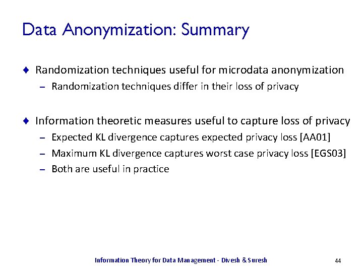
Data Anonymization: Summary ¨ Randomization techniques useful for microdata anonymization – Randomization techniques differ in their loss of privacy ¨ Information theoretic measures useful to capture loss of privacy Expected KL divergence captures expected privacy loss [AA 01] – Maximum KL divergence captures worst case privacy loss [EGS 03] – Both are useful in practice – Information Theory for Data Management - Divesh & Suresh 44

Outline Part 1 ¨ Introduction to Information Theory ¨ Application: Data Anonymization ¨ Application: Database Design Part 2 ¨ ¨ Review of Information Theory Basics Application: Data Integration Computing Information Theoretic Primitives Open Problems Information Theory for Data Management - Divesh & Suresh 45
![Information Dependencies DR 00 Goal use information theory to examine and reason about Information Dependencies [DR 00] ¨ Goal: use information theory to examine and reason about](https://slidetodoc.com/presentation_image_h/a9df4748910b2d014e3475a7d2f78649/image-46.jpg)
Information Dependencies [DR 00] ¨ Goal: use information theory to examine and reason about information content of the attributes in a relation instance ¨ Key ideas: Novel In. D measure between attribute sets X, Y based on H(Y|X) – Identify numeric inequalities between In. D measures – ¨ Results: In. D measures are a broader class than FDs and MVDs – Armstrong axioms for FDs derivable from In. D inequalities – MVD inference rules derivable from In. D inequalities – Information Theory for Data Management - Divesh & Suresh 46
![Information Dependencies DR 00 Functional dependency X Y FD X Information Dependencies [DR 00] ¨ Functional dependency: X → Y – FD X →](https://slidetodoc.com/presentation_image_h/a9df4748910b2d014e3475a7d2f78649/image-47.jpg)
Information Dependencies [DR 00] ¨ Functional dependency: X → Y – FD X → Y holds iff t 1, t 2 ((t 1[X] = t 2[X]) (t 1[Y] = t 2[Y])) X Y Z x 1 y 1 z 1 x 1 y 2 z 2 x 1 y 1 z 2 x 1 y 2 z 1 x 2 y 3 z 3 x 2 y 3 z 4 x 3 y 3 z 5 x 4 y 3 z 6 Information Theory for Data Management - Divesh & Suresh 47
![Information Dependencies DR 00 Functional dependency X Y FD X Information Dependencies [DR 00] ¨ Functional dependency: X → Y – FD X →](https://slidetodoc.com/presentation_image_h/a9df4748910b2d014e3475a7d2f78649/image-48.jpg)
Information Dependencies [DR 00] ¨ Functional dependency: X → Y – FD X → Y holds iff t 1, t 2 ((t 1[X] = t 2[X]) (t 1[Y] = t 2[Y])) X Y Z x 1 y 1 z 1 x 1 y 2 z 2 x 1 y 1 z 2 x 1 y 2 z 1 x 2 y 3 z 3 x 2 y 3 z 4 x 3 y 3 z 5 x 4 y 3 z 6 Information Theory for Data Management - Divesh & Suresh 48
![Information Dependencies DR 00 Result FD X Y holds iff HYX Information Dependencies [DR 00] ¨ Result: FD X → Y holds iff H(Y|X) =](https://slidetodoc.com/presentation_image_h/a9df4748910b2d014e3475a7d2f78649/image-49.jpg)
Information Dependencies [DR 00] ¨ Result: FD X → Y holds iff H(Y|X) = 0 – Intuition: once X is known, no remaining uncertainty in Y X Y p(X, Y) p(Y|X) h(Y|X) X p(X) x 1 y 1 0. 25 0. 5 1. 0 x 1 0. 5 x 1 y 2 0. 25 0. 5 1. 0 x 2 0. 25 x 2 y 3 0. 25 1. 0 0. 0 x 3 0. 125 x 3 y 3 0. 125 1. 0 0. 0 x 4 0. 125 x 4 y 3 0. 125 1. 0 0. 0 Y p(Y) y 1 0. 25 y 2 0. 25 y 3 0. 5 ¨ H(Y|X) = 0. 5 Information Theory for Data Management - Divesh & Suresh 49
![Information Dependencies DR 00 Multivalued dependency X Y MVD X Information Dependencies [DR 00] ¨ Multi-valued dependency: X →→ Y – MVD X →→](https://slidetodoc.com/presentation_image_h/a9df4748910b2d014e3475a7d2f78649/image-50.jpg)
Information Dependencies [DR 00] ¨ Multi-valued dependency: X →→ Y – MVD X →→ Y holds iff R(X, Y, Z) = R(X, Y) X Y Z x 1 y 1 z 1 x 1 y 2 z 2 x 1 y 1 z 2 x 1 y 2 z 1 x 2 y 3 z 3 x 2 y 3 z 4 x 3 y 3 z 5 x 4 y 3 z 6 R(X, Z) Information Theory for Data Management - Divesh & Suresh 50
![Information Dependencies DR 00 Multivalued dependency X Y MVD X Information Dependencies [DR 00] ¨ Multi-valued dependency: X →→ Y – MVD X →→](https://slidetodoc.com/presentation_image_h/a9df4748910b2d014e3475a7d2f78649/image-51.jpg)
Information Dependencies [DR 00] ¨ Multi-valued dependency: X →→ Y – MVD X →→ Y holds iff R(X, Y, Z) = R(X, Y) X Y Z X Y X Z x 1 y 1 z 1 x 1 y 1 x 1 z 1 x 1 y 2 z 2 x 1 y 2 x 1 z 2 x 1 y 1 z 2 x 2 y 3 x 2 z 3 x 1 y 2 z 1 x 3 y 3 x 2 z 4 x 2 y 3 z 3 x 4 y 3 x 3 z 5 x 2 y 3 z 4 x 4 z 6 x 3 y 3 z 5 x 4 y 3 z 6 = R(X, Z) Information Theory for Data Management - Divesh & Suresh 51
![Information Dependencies DR 00 Multivalued dependency X Y MVD X Information Dependencies [DR 00] ¨ Multi-valued dependency: X →→ Y – MVD X →→](https://slidetodoc.com/presentation_image_h/a9df4748910b2d014e3475a7d2f78649/image-52.jpg)
Information Dependencies [DR 00] ¨ Multi-valued dependency: X →→ Y – MVD X →→ Y holds iff R(X, Y, Z) = R(X, Y) X Y Z X Y X Z x 1 y 1 z 1 x 1 y 1 x 1 z 1 x 1 y 2 z 2 x 1 y 2 x 1 z 2 x 1 y 1 z 2 x 2 y 3 x 2 z 3 x 1 y 2 z 1 x 3 y 3 x 2 z 4 x 2 y 3 z 3 x 4 y 3 x 3 z 5 x 2 y 3 z 4 x 4 z 6 x 3 y 3 z 5 x 4 y 3 z 6 = R(X, Z) Information Theory for Data Management - Divesh & Suresh 52
![Information Dependencies DR 00 Result MVD X Y holds iff HY ZX Information Dependencies [DR 00] ¨ Result: MVD X →→ Y holds iff H(Y, Z|X)](https://slidetodoc.com/presentation_image_h/a9df4748910b2d014e3475a7d2f78649/image-53.jpg)
Information Dependencies [DR 00] ¨ Result: MVD X →→ Y holds iff H(Y, Z|X) = H(Y|X) + H(Z|X) – Intuition: once X known, uncertainties in Y and Z are independent X Y Z h(Y, Z|X) X Y h(Y|X) X Z h(Z|X) x 1 y 1 z 1 2. 0 x 1 y 1 1. 0 x 1 z 1 1. 0 x 1 y 2 z 2 2. 0 x 1 y 2 1. 0 x 1 z 2 1. 0 x 1 y 1 z 2 2. 0 x 2 y 3 0. 0 x 2 z 3 1. 0 x 1 y 2 z 1 2. 0 x 3 y 3 0. 0 x 2 z 4 1. 0 x 2 y 3 z 3 1. 0 x 4 y 3 0. 0 x 3 z 5 0. 0 x 2 y 3 z 4 1. 0 x 4 z 6 0. 0 x 3 y 3 z 5 0. 0 x 4 y 3 z 6 0. 0 = ¨ H(Y|X) = 0. 5, H(Z|X) = 0. 75, H(Y, Z|X) = 1. 25 Information Theory for Data Management - Divesh & Suresh 53
![Information Dependencies DR 00 Result Armstrong axioms for FDs derivable from In D Information Dependencies [DR 00] ¨ Result: Armstrong axioms for FDs derivable from In. D](https://slidetodoc.com/presentation_image_h/a9df4748910b2d014e3475a7d2f78649/image-54.jpg)
Information Dependencies [DR 00] ¨ Result: Armstrong axioms for FDs derivable from In. D inequalities ¨ Reflexivity: If Y X, then X → Y – H(Y|X) = 0 for Y X ¨ Augmentation: X → Y X, Z → Y, Z – 0 ≤ H(Y, Z|X, Z) = H(Y|X, Z) ≤ H(Y|X) = 0 ¨ Transitivity: X → Y & Y → Z X → Z – 0 ≥ H(Y|X) + H(Z|Y) ≥ H(Z|X) ≥ 0 Information Theory for Data Management - Divesh & Suresh 54

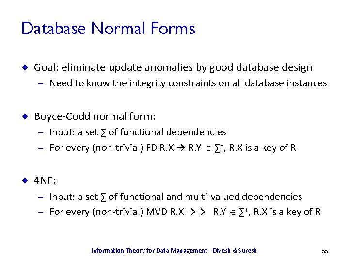
Database Normal Forms ¨ Goal: eliminate update anomalies by good database design – Need to know the integrity constraints on all database instances ¨ Boyce-Codd normal form: Input: a set ∑ of functional dependencies – For every (non-trivial) FD R. X → R. Y ∑+, R. X is a key of R – ¨ 4 NF: Input: a set ∑ of functional and multi-valued dependencies – For every (non-trivial) MVD R. X →→ R. Y ∑+, R. X is a key of R – Information Theory for Data Management - Divesh & Suresh 55

Database Normal Forms ¨ Functional dependency: X → Y – Which design is better? X Y Z X Y X Z x 1 y 1 z 1 x 1 y 1 x 1 z 1 x 1 y 1 z 2 x 2 y 2 x 1 z 2 x 2 y 2 z 3 x 3 y 3 x 2 z 3 x 2 y 2 z 4 x 4 y 4 x 2 z 4 x 3 y 3 z 5 x 4 y 4 z 6 x 4 z 6 = Information Theory for Data Management - Divesh & Suresh 56

Database Normal Forms ¨ Functional dependency: X → Y – Which design is better? X Y Z X Y X Z x 1 y 1 z 1 x 1 y 1 x 1 z 1 x 1 y 1 z 2 x 2 y 2 x 1 z 2 x 2 y 2 z 3 x 3 y 3 x 2 z 3 x 2 y 2 z 4 x 4 y 4 x 2 z 4 x 3 y 3 z 5 x 4 y 4 z 6 x 4 z 6 = ¨ Decomposition is in BCNF Information Theory for Data Management - Divesh & Suresh 57

Database Normal Forms ¨ Multi-valued dependency: X →→ Y – Which design is better? X Y Z X Y X Z x 1 y 1 z 1 x 1 y 1 x 1 z 1 x 1 y 2 z 2 x 1 y 2 x 1 z 2 x 1 y 1 z 2 x 2 y 3 x 2 z 3 x 1 y 2 z 1 x 3 y 3 x 2 z 4 x 2 y 3 z 3 x 4 y 3 x 3 z 5 x 2 y 3 z 4 x 4 z 6 x 3 y 3 z 5 x 4 y 3 z 6 = Information Theory for Data Management - Divesh & Suresh 58

Database Normal Forms ¨ Multi-valued dependency: X →→ Y – Which design is better? X Y Z X Y X Z x 1 y 1 z 1 x 1 y 1 x 1 z 1 x 1 y 2 z 2 x 1 y 2 x 1 z 2 x 1 y 1 z 2 x 2 y 3 x 2 z 3 x 1 y 2 z 1 x 3 y 3 x 2 z 4 x 2 y 3 z 3 x 4 y 3 x 3 z 5 x 2 y 3 z 4 x 4 z 6 x 3 y 3 z 5 x 4 y 3 z 6 = ¨ Decomposition is in 4 NF Information Theory for Data Management - Divesh & Suresh 59
![WellDesigned Databases AL 03 Goal use information theory to characterize goodness of a Well-Designed Databases [AL 03] ¨ Goal: use information theory to characterize “goodness” of a](https://slidetodoc.com/presentation_image_h/a9df4748910b2d014e3475a7d2f78649/image-60.jpg)
Well-Designed Databases [AL 03] ¨ Goal: use information theory to characterize “goodness” of a database design and reason about normalization algorithms ¨ Key idea: Information content measure of cell in a DB instance w. r. t. ICs – Redundancy reduces information content measure of cells – ¨ Results: Well-designed DB each cell has information content > 0 – Normalization algorithms never decrease information content – Information Theory for Data Management - Divesh & Suresh 60
![WellDesigned Databases AL 03 Information content of cell c in database D satisfying Well-Designed Databases [AL 03] ¨ Information content of cell c in database D satisfying](https://slidetodoc.com/presentation_image_h/a9df4748910b2d014e3475a7d2f78649/image-61.jpg)
Well-Designed Databases [AL 03] ¨ Information content of cell c in database D satisfying FD X → Y Uniform distribution p(V) on values for c consistent with Dc and FD – Information content of cell c is entropy H(V) – X Y Z V 62 p(V 62) h(V 62) x 1 y 1 z 1 y 1 0. 25 2. 0 x 1 y 1 z 2 y 2 0. 25 2. 0 x 2 y 2 z 3 y 3 0. 25 2. 0 x 2 y 2 z 4 y 4 0. 25 2. 0 x 3 y 3 z 5 x 4 y 4 z 6 ¨ H(V 62) = 2. 0 Information Theory for Data Management - Divesh & Suresh 61
![WellDesigned Databases AL 03 Information content of cell c in database D satisfying Well-Designed Databases [AL 03] ¨ Information content of cell c in database D satisfying](https://slidetodoc.com/presentation_image_h/a9df4748910b2d014e3475a7d2f78649/image-62.jpg)
Well-Designed Databases [AL 03] ¨ Information content of cell c in database D satisfying FD X → Y Uniform distribution p(V) on values for c consistent with Dc and FD – Information content of cell c is entropy H(V) – X Y Z V 22 p(V 22) h(V 22) x 1 y 1 z 1 y 1 1. 0 x 1 y 1 z 2 y 2 0. 0 x 2 y 2 z 3 y 3 0. 0 x 2 y 2 z 4 y 4 0. 0 x 3 y 3 z 5 x 4 y 4 z 6 0. 0 ¨ H(V 22) = 0. 0 Information Theory for Data Management - Divesh & Suresh 62
![WellDesigned Databases AL 03 Information content of cell c in database D satisfying Well-Designed Databases [AL 03] ¨ Information content of cell c in database D satisfying](https://slidetodoc.com/presentation_image_h/a9df4748910b2d014e3475a7d2f78649/image-63.jpg)
Well-Designed Databases [AL 03] ¨ Information content of cell c in database D satisfying FD X → Y – Information content of cell c is entropy H(V) X Y Z c H(V) x 1 y 1 z 1 c 12 0. 0 x 1 y 1 z 2 c 22 0. 0 x 2 y 2 z 3 c 32 0. 0 x 2 y 2 z 4 c 42 0. 0 x 3 y 3 z 5 c 52 2. 0 x 4 y 4 z 6 c 62 2. 0 ¨ Schema S is in BCNF iff D S, H(V) > 0, for all cells c in D – Technicalities w. r. t. size of active domain Information Theory for Data Management - Divesh & Suresh 63
![WellDesigned Databases AL 03 Information content of cell c in database D satisfying Well-Designed Databases [AL 03] ¨ Information content of cell c in database D satisfying](https://slidetodoc.com/presentation_image_h/a9df4748910b2d014e3475a7d2f78649/image-64.jpg)
Well-Designed Databases [AL 03] ¨ Information content of cell c in database D satisfying FD X → Y – Information content of cell c is entropy H(V) X Y X Z V 12 p(V 12) h(V 12) V 42 p(V 42) h(V 42) x 1 y 1 x 1 z 1 y 1 0. 25 2. 0 x 2 y 2 x 1 z 2 y 2 0. 25 2. 0 x 3 y 3 x 2 z 3 y 3 0. 25 2. 0 x 4 y 4 x 2 z 4 y 4 0. 25 2. 0 x 3 z 5 x 4 z 6 ¨ H(V 12) = 2. 0, H(V 42) = 2. 0 Information Theory for Data Management - Divesh & Suresh 64
![WellDesigned Databases AL 03 Information content of cell c in database D satisfying Well-Designed Databases [AL 03] ¨ Information content of cell c in database D satisfying](https://slidetodoc.com/presentation_image_h/a9df4748910b2d014e3475a7d2f78649/image-65.jpg)
Well-Designed Databases [AL 03] ¨ Information content of cell c in database D satisfying FD X → Y – Information content of cell c is entropy H(V) X Y X Z c H(V) x 1 y 1 x 1 z 1 c 12 2. 0 x 2 y 2 x 1 z 2 c 22 2. 0 x 3 y 3 x 2 z 3 c 32 2. 0 x 4 y 4 x 2 z 4 c 42 2. 0 x 3 z 5 x 4 z 6 ¨ Schema S is in BCNF iff D S, H(V) > 0, for all cells c in D Information Theory for Data Management - Divesh & Suresh 65
![WellDesigned Databases AL 03 Information content of cell c in DB D satisfying Well-Designed Databases [AL 03] ¨ Information content of cell c in DB D satisfying](https://slidetodoc.com/presentation_image_h/a9df4748910b2d014e3475a7d2f78649/image-66.jpg)
Well-Designed Databases [AL 03] ¨ Information content of cell c in DB D satisfying MVD X →→ Y – Information content of cell c is entropy H(V) X Y Z V 52 p(V 52) h(V 52) V 53 p(V 53) h(V 53) x 1 y 1 z 1 y 3 z 1 0. 2 2. 32 x 1 y 2 z 2 0. 2 2. 32 x 1 y 1 z 2 z 3 0. 2 2. 32 x 1 y 2 z 1 z 4 0. 0 x 2 y 3 z 5 0. 2 2. 32 x 2 y 3 z 4 z 6 0. 2 2. 32 x 3 y 3 z 5 x 4 y 3 z 6 1. 0 0. 0 ¨ H(V 52) = 0. 0, H(V 53) = 2. 32 Information Theory for Data Management - Divesh & Suresh 66
![WellDesigned Databases AL 03 Information content of cell c in DB D satisfying Well-Designed Databases [AL 03] ¨ Information content of cell c in DB D satisfying](https://slidetodoc.com/presentation_image_h/a9df4748910b2d014e3475a7d2f78649/image-67.jpg)
Well-Designed Databases [AL 03] ¨ Information content of cell c in DB D satisfying MVD X →→ Y – Information content of cell c is entropy H(V) X Y Z c H(V) x 1 y 1 z 1 c 12 0. 0 c 13 0. 0 x 1 y 2 z 2 c 22 0. 0 c 23 0. 0 x 1 y 1 z 2 c 32 0. 0 c 33 0. 0 x 1 y 2 z 1 c 42 0. 0 c 43 0. 0 x 2 y 3 z 3 c 52 0. 0 c 53 2. 32 x 2 y 3 z 4 c 62 0. 0 c 63 2. 32 x 3 y 3 z 5 c 72 1. 58 c 73 2. 58 x 4 y 3 z 6 c 82 1. 58 c 83 2. 58 ¨ Schema S is in 4 NF iff D S, H(V) > 0, for all cells c in D Information Theory for Data Management - Divesh & Suresh 67
![WellDesigned Databases AL 03 Information content of cell c in DB D satisfying Well-Designed Databases [AL 03] ¨ Information content of cell c in DB D satisfying](https://slidetodoc.com/presentation_image_h/a9df4748910b2d014e3475a7d2f78649/image-68.jpg)
Well-Designed Databases [AL 03] ¨ Information content of cell c in DB D satisfying MVD X →→ Y – Information content of cell c is entropy H(V) X Y X Z V 32 p(V 32) h(V 32) V 34 p(V 34) h(V 34) x 1 y 1 x 1 z 1 y 1 0. 33 1. 58 z 1 0. 2 2. 32 x 1 y 2 x 1 z 2 y 2 0. 33 1. 58 z 2 0. 2 2. 32 x 2 y 3 x 2 z 3 y 3 0. 33 1. 58 z 3 0. 2 2. 32 x 3 y 3 x 2 z 4 0. 0 x 4 y 3 x 3 z 5 0. 2 2. 32 x 4 z 6 0. 2 2. 32 ¨ H(V 32) = 1. 58, H(V 34) = 2. 32 Information Theory for Data Management - Divesh & Suresh 68
![WellDesigned Databases AL 03 Information content of cell c in DB D satisfying Well-Designed Databases [AL 03] ¨ Information content of cell c in DB D satisfying](https://slidetodoc.com/presentation_image_h/a9df4748910b2d014e3475a7d2f78649/image-69.jpg)
Well-Designed Databases [AL 03] ¨ Information content of cell c in DB D satisfying MVD X →→ Y – Information content of cell c is entropy H(V) X Y X Z c H(V) x 1 y 1 x 1 z 1 c 12 1. 0 c 14 2. 32 x 1 y 2 x 1 z 2 c 22 1. 0 c 24 2. 32 x 2 y 3 x 2 z 3 c 32 1. 58 c 34 2. 32 x 3 y 3 x 2 z 4 c 42 1. 58 c 44 2. 32 x 4 y 3 x 3 z 5 c 52 1. 58 c 54 2. 58 x 4 z 6 c 64 2. 58 ¨ Schema S is in 4 NF iff D S, H(V) > 0, for all cells c in D Information Theory for Data Management - Divesh & Suresh 69
![WellDesigned Databases AL 03 Normalization algorithms never decrease information content Information content Well-Designed Databases [AL 03] ¨ Normalization algorithms never decrease information content – Information content](https://slidetodoc.com/presentation_image_h/a9df4748910b2d014e3475a7d2f78649/image-70.jpg)
Well-Designed Databases [AL 03] ¨ Normalization algorithms never decrease information content – Information content of cell c is entropy H(V) X Y Z c H(V) x 1 y 1 z 1 c 13 0. 0 x 1 y 2 z 2 c 23 0. 0 x 1 y 1 z 2 c 33 0. 0 x 1 y 2 z 1 c 43 0. 0 x 2 y 3 z 3 c 53 2. 32 x 2 y 3 z 4 c 63 2. 32 x 3 y 3 z 5 c 73 2. 58 x 4 y 3 z 6 c 83 2. 58 Information Theory for Data Management - Divesh & Suresh 70
![WellDesigned Databases AL 03 Normalization algorithms never decrease information content Information content Well-Designed Databases [AL 03] ¨ Normalization algorithms never decrease information content – Information content](https://slidetodoc.com/presentation_image_h/a9df4748910b2d014e3475a7d2f78649/image-71.jpg)
Well-Designed Databases [AL 03] ¨ Normalization algorithms never decrease information content – Information content of cell c is entropy H(V) X Y Z X Y X Z c H(V) x 1 y 1 z 1 x 1 y 1 x 1 z 1 c 13 0. 0 c 14 2. 32 x 1 y 2 z 2 x 1 y 2 x 1 z 2 c 23 0. 0 c 24 2. 32 x 1 y 1 z 2 x 2 y 3 x 2 z 3 c 33 0. 0 c 34 2. 32 x 1 y 2 z 1 x 3 y 3 x 2 z 4 c 43 0. 0 c 44 2. 32 x 2 y 3 z 3 x 4 y 3 x 3 z 5 c 53 2. 32 c 54 2. 58 x 2 y 3 z 4 x 4 z 6 c 63 2. 32 c 64 2. 58 x 3 y 3 z 5 c 73 2. 58 x 4 y 3 z 6 c 83 2. 58 = Information Theory for Data Management - Divesh & Suresh 71
![WellDesigned Databases AL 03 Normalization algorithms never decrease information content Information content Well-Designed Databases [AL 03] ¨ Normalization algorithms never decrease information content – Information content](https://slidetodoc.com/presentation_image_h/a9df4748910b2d014e3475a7d2f78649/image-72.jpg)
Well-Designed Databases [AL 03] ¨ Normalization algorithms never decrease information content – Information content of cell c is entropy H(V) X Y Z X Y X Z c H(V) x 1 y 1 z 1 x 1 y 1 x 1 z 1 c 13 0. 0 c 14 2. 32 x 1 y 2 z 2 x 1 y 2 x 1 z 2 c 23 0. 0 c 24 2. 32 x 1 y 1 z 2 x 2 y 3 x 2 z 3 c 33 0. 0 c 34 2. 32 x 1 y 2 z 1 x 3 y 3 x 2 z 4 c 43 0. 0 c 44 2. 32 x 2 y 3 z 3 x 4 y 3 x 3 z 5 c 53 2. 32 c 54 2. 58 x 2 y 3 z 4 x 4 z 6 c 63 2. 32 c 64 2. 58 x 3 y 3 z 5 c 73 2. 58 x 4 y 3 z 6 c 83 2. 58 = Information Theory for Data Management - Divesh & Suresh 72

Database Design: Summary ¨ Good database design essential for preserving data integrity ¨ Information theoretic measures useful for integrity constraints FD X → Y holds iff In. D measure H(Y|X) = 0 – MVD X →→ Y holds iff H(Y, Z|X) = H(Y|X) + H(Z|X) – Information theory to model correlations in specific database – ¨ Information theoretic measures useful for normal forms Schema S is in BCNF/4 NF iff D S, H(V) > 0, for all cells c in D – Information theory to model distributions over possible databases – Information Theory for Data Management - Divesh & Suresh 73

Outline Part 1 ¨ Introduction to Information Theory ¨ Application: Data Anonymization ¨ Application: Database Design Part 2 ¨ ¨ Review of Information Theory Basics Application: Data Integration Computing Information Theoretic Primitives Open Problems Information Theory for Data Management - Divesh & Suresh 74

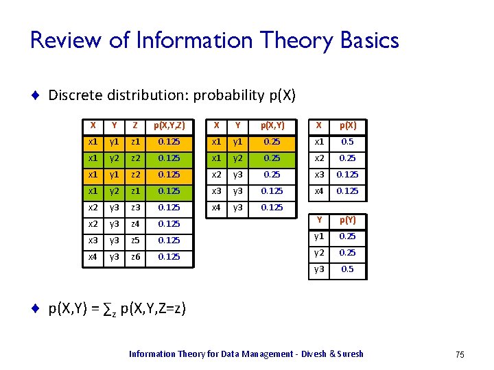
Review of Information Theory Basics ¨ Discrete distribution: probability p(X) X Y Z p(X, Y, Z) X Y p(X, Y) X p(X) x 1 y 1 z 1 0. 125 x 1 y 1 0. 25 x 1 0. 5 x 1 y 2 z 2 0. 125 x 1 y 2 0. 25 x 1 y 1 z 2 0. 125 x 2 y 3 0. 25 x 3 0. 125 x 1 y 2 z 1 0. 125 x 3 y 3 0. 125 x 4 0. 125 x 2 y 3 z 3 0. 125 x 4 y 3 0. 125 x 2 y 3 z 4 0. 125 Y p(Y) x 3 y 3 z 5 0. 125 y 1 0. 25 x 4 y 3 z 6 0. 125 y 2 0. 25 y 3 0. 5 ¨ p(X, Y) = ∑z p(X, Y, Z=z) Information Theory for Data Management - Divesh & Suresh 75

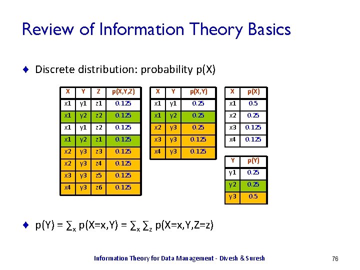
Review of Information Theory Basics ¨ Discrete distribution: probability p(X) X Y Z p(X, Y, Z) X Y p(X, Y) X p(X) x 1 y 1 z 1 0. 125 x 1 y 1 0. 25 x 1 0. 5 x 1 y 2 z 2 0. 125 x 1 y 2 0. 25 x 1 y 1 z 2 0. 125 x 2 y 3 0. 25 x 3 0. 125 x 1 y 2 z 1 0. 125 x 3 y 3 0. 125 x 4 0. 125 x 2 y 3 z 3 0. 125 x 4 y 3 0. 125 x 2 y 3 z 4 0. 125 Y p(Y) x 3 y 3 z 5 0. 125 y 1 0. 25 x 4 y 3 z 6 0. 125 y 2 0. 25 y 3 0. 5 ¨ p(Y) = ∑x p(X=x, Y) = ∑x ∑z p(X=x, Y, Z=z) Information Theory for Data Management - Divesh & Suresh 76

Review of Information Theory Basics ¨ Discrete distribution: conditional probability p(X|Y) X Y p(X, Y) p(X|Y) p(Y|X) X p(X) x 1 y 1 0. 25 1. 0 0. 5 x 1 y 2 0. 25 1. 0 0. 5 x 2 0. 25 x 2 y 3 0. 25 0. 5 1. 0 x 3 0. 125 x 3 y 3 0. 125 0. 25 1. 0 x 4 0. 125 x 4 y 3 0. 125 0. 25 1. 0 Y p(Y) y 1 0. 25 y 2 0. 25 y 3 0. 5 ¨ p(X, Y) = p(X|Y)*p(Y) = p(Y|X)*p(X) Information Theory for Data Management - Divesh & Suresh 77

Review of Information Theory Basics ¨ Discrete distribution: entropy H(X) X Y p(X, Y) h(X, Y) X p(X) h(X) x 1 y 1 0. 25 2. 0 x 1 0. 5 1. 0 x 1 y 2 0. 25 2. 0 x 2 y 3 0. 25 2. 0 x 3 0. 125 3. 0 x 3 y 3 0. 125 3. 0 x 4 y 3 0. 125 3. 0 Y p(Y) h(Y) y 1 0. 25 2. 0 y 2 0. 25 2. 0 y 3 0. 5 1. 0 ¨ h(x) = log 2(1/p(x)) H(X) = ∑X=x p(x)*h(x) = 1. 75 – H(Y) = ∑Y=y p(y)*h(y) = 1. 5 (≤ log 2(|Y|) = 1. 58) – H(X, Y) = ∑X=x ∑Y=y p(x, y)*h(x, y) = 2. 25 (≤ log 2(|X, Y|) = 2. 32) – Information Theory for Data Management - Divesh & Suresh 78

Review of Information Theory Basics ¨ Discrete distribution: conditional entropy H(X|Y) X Y p(X, Y) p(X|Y) h(X|Y) X p(X) h(X) x 1 y 1 0. 25 1. 0 0. 0 x 1 0. 5 1. 0 x 1 y 2 0. 25 1. 0 0. 0 x 2 0. 25 2. 0 x 2 y 3 0. 25 0. 5 1. 0 x 3 0. 125 3. 0 x 3 y 3 0. 125 0. 25 2. 0 x 4 0. 125 3. 0 x 4 y 3 0. 125 0. 25 2. 0 Y p(Y) h(Y) y 1 0. 25 2. 0 y 2 0. 25 2. 0 y 3 0. 5 1. 0 ¨ h(x|y) = log 2(1/p(x|y)) H(X|Y) = ∑X=x ∑Y=y p(x, y)*h(x|y) = 0. 75 – H(X|Y) = H(X, Y) – H(Y) = 2. 25 – 1. 5 – Information Theory for Data Management - Divesh & Suresh 79

Review of Information Theory Basics ¨ Discrete distribution: mutual information I(X; Y) X Y p(X, Y) h(X, Y) i(X; Y) X p(X) h(X) x 1 y 1 0. 25 2. 0 1. 0 x 1 0. 5 1. 0 x 1 y 2 0. 25 2. 0 1. 0 x 2 0. 25 2. 0 x 2 y 3 0. 25 2. 0 1. 0 x 3 0. 125 3. 0 x 3 y 3 0. 125 3. 0 1. 0 x 4 0. 125 3. 0 x 4 y 3 0. 125 3. 0 1. 0 Y p(Y) h(Y) y 1 0. 25 2. 0 y 2 0. 25 2. 0 y 3 0. 5 1. 0 ¨ i(x; y) = log 2(p(x, y)/p(x)*p(y)) I(X; Y) = ∑X=x ∑Y=y p(x, y)*i(x; y) = 1. 0 – I(X; Y) = H(X) + H(Y) – H(X, Y) = 1. 75 + 1. 5 – 2. 25 – Information Theory for Data Management - Divesh & Suresh 80

Outline Part 1 ¨ Introduction to Information Theory ¨ Application: Data Anonymization ¨ Application: Database Design Part 2 ¨ ¨ Review of Information Theory Basics Application: Data Integration Computing Information Theoretic Primitives Open Problems Information Theory for Data Management - Divesh & Suresh 81

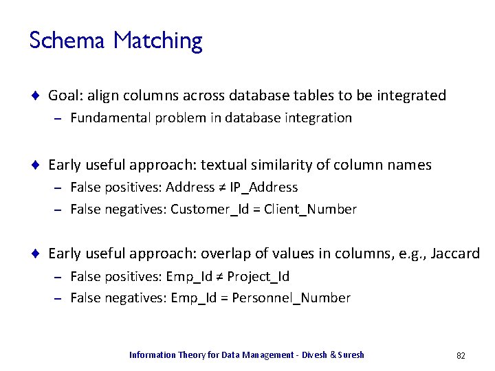
Schema Matching ¨ Goal: align columns across database tables to be integrated – Fundamental problem in database integration ¨ Early useful approach: textual similarity of column names False positives: Address ≠ IP_Address – False negatives: Customer_Id = Client_Number – ¨ Early useful approach: overlap of values in columns, e. g. , Jaccard False positives: Emp_Id ≠ Project_Id – False negatives: Emp_Id = Personnel_Number – Information Theory for Data Management - Divesh & Suresh 82
![Opaque Schema Matching KN 03 Goal align columns when column names data values Opaque Schema Matching [KN 03] ¨ Goal: align columns when column names, data values](https://slidetodoc.com/presentation_image_h/a9df4748910b2d014e3475a7d2f78649/image-83.jpg)
Opaque Schema Matching [KN 03] ¨ Goal: align columns when column names, data values are opaque Databases belong to different government bureaucracies – Treat column names and data values as uninterpreted (generic) – A B C D W X Y Z a 1 b 2 c 1 d 1 w 2 x 1 y 1 z 2 a 3 b 4 c 2 d 2 w 4 x 2 y 3 z 3 a 1 b 1 c 1 d 2 w 3 x 3 y 3 z 1 a 4 b 3 c 2 d 3 w 1 x 2 y 1 z 2 ¨ Example: EMP_PROJ(Emp_Id, Proj_Id, Task_Id, Status_Id) Likely that all Id fields are from the same domain – Different databases may have different column names – Information Theory for Data Management - Divesh & Suresh 83
![Opaque Schema Matching KN 03 Approach build complete labeled graph GD for each Opaque Schema Matching [KN 03] ¨ Approach: build complete, labeled graph GD for each](https://slidetodoc.com/presentation_image_h/a9df4748910b2d014e3475a7d2f78649/image-84.jpg)
Opaque Schema Matching [KN 03] ¨ Approach: build complete, labeled graph GD for each database D Nodes are columns, label(node(X)) = H(X), label(edge(X, Y)) = I(X; Y) – Perform graph matching between GD 1 and GD 2, minimizing distance – ¨ Intuition: Entropy H(X) captures distribution of values in database column X – Mutual information I(X; Y) captures correlations between X, Y – Efficiency: graph matching between schema-sized graphs – Information Theory for Data Management - Divesh & Suresh 84
![Opaque Schema Matching KN 03 Approach build complete labeled graph GD for each Opaque Schema Matching [KN 03] ¨ Approach: build complete, labeled graph GD for each](https://slidetodoc.com/presentation_image_h/a9df4748910b2d014e3475a7d2f78649/image-85.jpg)
Opaque Schema Matching [KN 03] ¨ Approach: build complete, labeled graph GD for each database D – Nodes are columns, label(node(X)) = H(X), label(edge(X, Y)) = I(X; Y) A B C D A p(A) B p(B) C p(C) D p(D) a 1 b 2 c 1 d 1 a 1 0. 5 b 1 0. 25 c 1 0. 5 d 1 0. 25 a 3 b 4 c 2 d 2 a 3 0. 25 b 2 0. 25 c 2 0. 5 d 2 0. 5 a 1 b 1 c 1 d 2 a 4 0. 25 b 3 0. 25 d 3 0. 25 a 4 b 3 c 2 d 3 b 4 0. 25 Information Theory for Data Management - Divesh & Suresh 85
![Opaque Schema Matching KN 03 Approach build complete labeled graph GD for each Opaque Schema Matching [KN 03] ¨ Approach: build complete, labeled graph GD for each](https://slidetodoc.com/presentation_image_h/a9df4748910b2d014e3475a7d2f78649/image-86.jpg)
Opaque Schema Matching [KN 03] ¨ Approach: build complete, labeled graph GD for each database D – Nodes are columns, label(node(X)) = H(X), label(edge(X, Y)) = I(X; Y) A B C D A h(A) B h(B) C h(C) D h(D) a 1 b 2 c 1 d 1 a 1 1. 0 b 1 2. 0 c 1 1. 0 d 1 2. 0 a 3 b 4 c 2 d 2 a 3 2. 0 b 2 2. 0 c 2 1. 0 d 2 1. 0 a 1 b 1 c 1 d 2 a 4 2. 0 b 3 2. 0 d 3 2. 0 a 4 b 3 c 2 d 3 b 4 2. 0 ¨ H(A) = 1. 5, H(B) = 2. 0, H(C) = 1. 0, H(D) = 1. 5 Information Theory for Data Management - Divesh & Suresh 86
![Opaque Schema Matching KN 03 Approach build complete labeled graph GD for each Opaque Schema Matching [KN 03] ¨ Approach: build complete, labeled graph GD for each](https://slidetodoc.com/presentation_image_h/a9df4748910b2d014e3475a7d2f78649/image-87.jpg)
Opaque Schema Matching [KN 03] ¨ Approach: build complete, labeled graph GD for each database D – Nodes are columns, label(node(X)) = H(X), label(edge(X, Y)) = I(X; Y) A B C D A h(A) B h(B) A B h(A, B) i(A; B) a 1 b 2 c 1 d 1 a 1 1. 0 b 1 2. 0 a 1 b 2 2. 0 1. 0 a 3 b 4 c 2 d 2 a 3 2. 0 b 2 2. 0 a 3 b 4 2. 0 a 1 b 1 c 1 d 2 a 4 2. 0 b 3 2. 0 a 1 b 1 2. 0 1. 0 a 4 b 3 c 2 d 3 b 4 2. 0 a 4 b 3 2. 0 ¨ H(A) = 1. 5, H(B) = 2. 0, H(C) = 1. 0, H(D) = 1. 5, I(A; B) = 1. 5 Information Theory for Data Management - Divesh & Suresh 87
![Opaque Schema Matching KN 03 Approach build complete labeled graph GD for each Opaque Schema Matching [KN 03] ¨ Approach: build complete, labeled graph GD for each](https://slidetodoc.com/presentation_image_h/a9df4748910b2d014e3475a7d2f78649/image-88.jpg)
Opaque Schema Matching [KN 03] ¨ Approach: build complete, labeled graph GD for each database D – Nodes are columns, label(node(X)) = H(X), label(edge(X, Y)) = I(X; Y) A B C D a 1 b 2 c 1 d 1 a 3 b 4 c 2 d 2 a 1 b 1 c 1 d 2 a 4 b 3 c 2 d 3 1. 5 A B 2. 0 1. 5 1. 0 C D 1. 5 0. 5 Information Theory for Data Management - Divesh & Suresh 88
![Opaque Schema Matching KN 03 Approach build complete labeled graph GD for each Opaque Schema Matching [KN 03] ¨ Approach: build complete, labeled graph GD for each](https://slidetodoc.com/presentation_image_h/a9df4748910b2d014e3475a7d2f78649/image-89.jpg)
Opaque Schema Matching [KN 03] ¨ Approach: build complete, labeled graph GD for each database D Nodes are columns, label(node(X)) = H(X), label(edge(X, Y)) = I(X; Y) – Perform graph matching between GD 1 and GD 2, minimizing distance – 1. 5 A B 2. 0 1. 0 X 1. 5 1. 0 1. 5 W 0. 5 C D 0. 5 1. 0 Y Z 1. 5 1. 0 ¨ [KN 03] uses euclidean and normal distance metrics Information Theory for Data Management - Divesh & Suresh 89
![Opaque Schema Matching KN 03 Approach build complete labeled graph GD for each Opaque Schema Matching [KN 03] ¨ Approach: build complete, labeled graph GD for each](https://slidetodoc.com/presentation_image_h/a9df4748910b2d014e3475a7d2f78649/image-90.jpg)
Opaque Schema Matching [KN 03] ¨ Approach: build complete, labeled graph GD for each database D Nodes are columns, label(node(X)) = H(X), label(edge(X, Y)) = I(X; Y) – Perform graph matching between GD 1 and GD 2, minimizing distance – 1. 5 A B 2. 0 1. 0 X 1. 5 1. 0 1. 5 W 0. 5 C D 0. 5 1. 0 Y Z 1. 5 1. 0 Information Theory for Data Management - Divesh & Suresh 90
![Opaque Schema Matching KN 03 Approach build complete labeled graph GD for each Opaque Schema Matching [KN 03] ¨ Approach: build complete, labeled graph GD for each](https://slidetodoc.com/presentation_image_h/a9df4748910b2d014e3475a7d2f78649/image-91.jpg)
Opaque Schema Matching [KN 03] ¨ Approach: build complete, labeled graph GD for each database D Nodes are columns, label(node(X)) = H(X), label(edge(X, Y)) = I(X; Y) – Perform graph matching between GD 1 and GD 2, minimizing distance – 1. 5 A B 2. 0 1. 0 X 1. 5 1. 0 1. 5 W 0. 5 C D 0. 5 1. 0 Y Z 1. 5 1. 0 Information Theory for Data Management - Divesh & Suresh 91
![Heterogeneity Identification DKOSV 06 Goal identify columns with semantically heterogeneous values Can Heterogeneity Identification [DKOSV 06] ¨ Goal: identify columns with semantically heterogeneous values – Can](https://slidetodoc.com/presentation_image_h/a9df4748910b2d014e3475a7d2f78649/image-92.jpg)
Heterogeneity Identification [DKOSV 06] ¨ Goal: identify columns with semantically heterogeneous values – Can arise due to opaque schema matching [KN 03] ¨ Key ideas: Heterogeneity based on distribution, distinguishability of values – Use Information Theory to quantify heterogeneity – ¨ Issues: Which information theoretic measure characterizes heterogeneity? – How do we actually cluster the data ? – Information Theory for Data Management - Divesh & Suresh 92
![Heterogeneity Identification DKOSV 06 Example semantically homogeneous heterogeneous columns CustomerId h 8742yyy com Heterogeneity Identification [DKOSV 06] ¨ Example: semantically homogeneous, heterogeneous columns Customer_Id h 8742@yyy. com](https://slidetodoc.com/presentation_image_h/a9df4748910b2d014e3475a7d2f78649/image-93.jpg)
Heterogeneity Identification [DKOSV 06] ¨ Example: semantically homogeneous, heterogeneous columns Customer_Id h 8742@yyy. com kkjj+@haha. org qwerty@keyboard. us 555 -1212@fax. in alpha@beta. ga (908)-555 -1234 john. smith@noname. org 973 -360 -0000 jane. doe@1973 law. us 360 -0007 jamesbond. 007@action. com (877)-807 -4596 Information Theory for Data Management - Divesh & Suresh 93
![Heterogeneity Identification DKOSV 06 Example semantically homogeneous heterogeneous columns CustomerId h 8742yyy com Heterogeneity Identification [DKOSV 06] ¨ Example: semantically homogeneous, heterogeneous columns Customer_Id h 8742@yyy. com](https://slidetodoc.com/presentation_image_h/a9df4748910b2d014e3475a7d2f78649/image-94.jpg)
Heterogeneity Identification [DKOSV 06] ¨ Example: semantically homogeneous, heterogeneous columns Customer_Id h 8742@yyy. com kkjj+@haha. org qwerty@keyboard. us 555 -1212@fax. in alpha@beta. ga (908)-555 -1234 john. smith@noname. org 973 -360 -0000 jane. doe@1973 law. us 360 -0007 jamesbond. 007@action. com (877)-807 -4596 Information Theory for Data Management - Divesh & Suresh 94
![Heterogeneity Identification DKOSV 06 Example semantically homogeneous heterogeneous columns CustomerId h 8742yyy com Heterogeneity Identification [DKOSV 06] ¨ Example: semantically homogeneous, heterogeneous columns Customer_Id h 8742@yyy. com](https://slidetodoc.com/presentation_image_h/a9df4748910b2d014e3475a7d2f78649/image-95.jpg)
Heterogeneity Identification [DKOSV 06] ¨ Example: semantically homogeneous, heterogeneous columns Customer_Id h 8742@yyy. com kkjj+@haha. org qwerty@keyboard. us 555 -1212@fax. in alpha@beta. ga (908)-555 -1234 john. smith@noname. org 973 -360 -0000 jane. doe@1973 law. us 360 -0007 jamesbond. 007@action. com (877)-807 -4596 ¨ More semantic types in column greater heterogeneity – Only email versus email + phone Information Theory for Data Management - Divesh & Suresh 95
![Heterogeneity Identification DKOSV 06 Example semantically homogeneous heterogeneous columns CustomerId h 8742yyy com Heterogeneity Identification [DKOSV 06] ¨ Example: semantically homogeneous, heterogeneous columns Customer_Id h 8742@yyy. com](https://slidetodoc.com/presentation_image_h/a9df4748910b2d014e3475a7d2f78649/image-96.jpg)
Heterogeneity Identification [DKOSV 06] ¨ Example: semantically homogeneous, heterogeneous columns Customer_Id h 8742@yyy. com kkjj+@haha. org qwerty@keyboard. us 555 -1212@fax. in alpha@beta. ga (908)-555 -1234 john. smith@noname. org 973 -360 -0000 jane. doe@1973 law. us 360 -0007 (877)-807 -4596 Information Theory for Data Management - Divesh & Suresh 96
![Heterogeneity Identification DKOSV 06 Example semantically homogeneous heterogeneous columns CustomerId h 8742yyy com Heterogeneity Identification [DKOSV 06] ¨ Example: semantically homogeneous, heterogeneous columns Customer_Id h 8742@yyy. com](https://slidetodoc.com/presentation_image_h/a9df4748910b2d014e3475a7d2f78649/image-97.jpg)
Heterogeneity Identification [DKOSV 06] ¨ Example: semantically homogeneous, heterogeneous columns Customer_Id h 8742@yyy. com kkjj+@haha. org qwerty@keyboard. us 555 -1212@fax. in alpha@beta. ga (908)-555 -1234 john. smith@noname. org 973 -360 -0000 jane. doe@1973 law. us 360 -0007 (877)-807 -4596 ¨ Relative distribution of semantic types impacts heterogeneity – Mainly email + few phone versus balanced email + phone Information Theory for Data Management - Divesh & Suresh 97
![Heterogeneity Identification DKOSV 06 Example semantically homogeneous heterogeneous columns CustomerId 187 65 2468 Heterogeneity Identification [DKOSV 06] ¨ Example: semantically homogeneous, heterogeneous columns Customer_Id 187 -65 -2468](https://slidetodoc.com/presentation_image_h/a9df4748910b2d014e3475a7d2f78649/image-98.jpg)
Heterogeneity Identification [DKOSV 06] ¨ Example: semantically homogeneous, heterogeneous columns Customer_Id 187 -65 -2468 h 8742@yyy. com 987 -64 -6837 kkjj+@haha. org 789 -15 -4321 qwerty@keyboard. us 987 -65 -4321 555 -1212@fax. in (908)-555 -1234 973 -360 -0000 360 -0007 (877)-807 -4596 Information Theory for Data Management - Divesh & Suresh 98
![Heterogeneity Identification DKOSV 06 Example semantically homogeneous heterogeneous columns CustomerId 187 65 2468 Heterogeneity Identification [DKOSV 06] ¨ Example: semantically homogeneous, heterogeneous columns Customer_Id 187 -65 -2468](https://slidetodoc.com/presentation_image_h/a9df4748910b2d014e3475a7d2f78649/image-99.jpg)
Heterogeneity Identification [DKOSV 06] ¨ Example: semantically homogeneous, heterogeneous columns Customer_Id 187 -65 -2468 h 8742@yyy. com 987 -64 -6837 kkjj+@haha. org 789 -15 -4321 qwerty@keyboard. us 987 -65 -4321 555 -1212@fax. in (908)-555 -1234 973 -360 -0000 360 -0007 (877)-807 -4596 Information Theory for Data Management - Divesh & Suresh 99
![Heterogeneity Identification DKOSV 06 Example semantically homogeneous heterogeneous columns CustomerId 187 65 2468 Heterogeneity Identification [DKOSV 06] ¨ Example: semantically homogeneous, heterogeneous columns Customer_Id 187 -65 -2468](https://slidetodoc.com/presentation_image_h/a9df4748910b2d014e3475a7d2f78649/image-100.jpg)
Heterogeneity Identification [DKOSV 06] ¨ Example: semantically homogeneous, heterogeneous columns Customer_Id 187 -65 -2468 h 8742@yyy. com 987 -64 -6837 kkjj+@haha. org 789 -15 -4321 qwerty@keyboard. us 987 -65 -4321 555 -1212@fax. in (908)-555 -1234 973 -360 -0000 360 -0007 (877)-807 -4596 ¨ More easily distinguished types greater heterogeneity – Phone + (possibly) SSN versus balanced email + phone Information Theory for Data Management - Divesh & Suresh 100
![Heterogeneity Identification DKOSV 06 Heterogeneity complexity of describing the data Heterogeneity Identification [DKOSV 06] ¨ Heterogeneity = complexity of describing the data – –](https://slidetodoc.com/presentation_image_h/a9df4748910b2d014e3475a7d2f78649/image-101.jpg)
Heterogeneity Identification [DKOSV 06] ¨ Heterogeneity = complexity of describing the data – – More, balanced clusters greater heterogeneity More distinguishable clusters greater heterogeneity ¨ Use two views of mutual information It quantifies the complexity of describing the data (compression) 2. It quantifies the quality of the compression 1. Information Theory for Data Management - Divesh & Suresh 101
![Heterogeneity Identification DKOSV 06 Hard clustering X CustomerId T ClusterId 187 Heterogeneity Identification [DKOSV 06] ¨ Hard clustering X = Customer_Id T = Cluster_Id 187](https://slidetodoc.com/presentation_image_h/a9df4748910b2d014e3475a7d2f78649/image-102.jpg)
Heterogeneity Identification [DKOSV 06] ¨ Hard clustering X = Customer_Id T = Cluster_Id 187 -65 -2468 t 1 987 -64 -6837 t 1 789 -15 -4321 t 1 987 -65 -4321 t 1 (908)-555 -1234 t 2 973 -360 -0000 t 1 360 -0007 t 3 (877)-807 -4596 t 2 Information Theory for Data Management - Divesh & Suresh 102

Measuring complexity of clustering ¨ Take 1: complexity of a clustering = #clusters – standard model of complexity. ¨ Doesn’t capture the fact that clusters have different sizes. Information Theory for Data Management - Divesh & Suresh 103

Measuring complexity of clustering ¨ Take 2: Complexity of clustering = number of bits needed to describe it. ¨ Writing down “k” needs log k bits. ¨ In general, let cluster t T have |t| elements. set p(t) = |t|/n – #bits to write down cluster sizes = H(T) = S pt log 1/pt – H( ) < H( Information Theory for Data Management - Divesh & Suresh ) 104
![Heterogeneity Identification DKOSV 06 Soft clustering cluster membership probabilities X CustomerId T Heterogeneity Identification [DKOSV 06] ¨ Soft clustering: cluster membership probabilities X = Customer_Id T](https://slidetodoc.com/presentation_image_h/a9df4748910b2d014e3475a7d2f78649/image-105.jpg)
Heterogeneity Identification [DKOSV 06] ¨ Soft clustering: cluster membership probabilities X = Customer_Id T = Cluster_Id p(T|X) 789 -15 -4321 t 1 0. 75 987 -65 -4321 t 1 0. 75 789 -15 -4321 t 2 0. 25 987 -65 -4321 t 2 0. 25 (908)-555 -1234 t 1 0. 25 973 -360 -0000 t 1 0. 5 (908)-555 -1234 t 2 0. 75 973 -360 -0000 t 2 0. 5 ¨ How to compute a good soft clustering? Information Theory for Data Management - Divesh & Suresh 105

Measuring complexity of clustering ¨ Take 1: p(t) = Sx p(x) p(t|x) – Compute H(T) as before. – ¨ Problem: T 1 t 2 T 2 t 1 t 2 x 1 0. 5 x 1 0. 99 0. 01 x 2 0. 5 x 2 0. 01 0. 99 h(T) 0. 5 H(T 1) = H(T 2) !! Information Theory for Data Management - Divesh & Suresh 106

Measuring complexity of clustering ¨ By averaging the memberships, we’ve lost useful information. ¨ Take II: Compute I(T; X) ! X T 1 p(X, T) i(X; T) X T 2 p(X, T) i(X; T) x 1 t 1 0. 25 0 x 1 t 1 0. 495 0. 99 x 1 t 2 0. 25 0 x 1 t 2 0. 005 -5. 64 x 2 t 1 0. 25 0 x 2 t 2 0. 25 0 I(T 1; X) = 0 I(T 2; X) = 0. 46 ¨ Even better: If T is a hard clustering of X, then I(T; X) = H(T) Information Theory for Data Management - Divesh & Suresh 107

Measuring cost of a cluster Given objects Xt = {X 1, X 2, …, Xm} in cluster t, Cost(t) = sum of distances from Xi to cluster center If we set distance to be KL-distance, then Cost of a cluster = I(X t, V) Information Theory for Data Management - Divesh & Suresh 108

Cost of a clustering ¨ If we partition X into k clusters X 1, . . . , Xk ¨ Cost(clustering) = Si pi I(Xi, V) (pi = |Xi|/|X|) ¨ Suppose we treat each cluster center itself as a point ? Information Theory for Data Management - Divesh & Suresh 109

Cost of a clustering ¨ We can write down the “cost” of this “cluster” – Cost(T) = I(T; V) ¨ Key result [BMDG 05] : Cost(clustering) = I(X, V) – I(T, V) Minimizing cost(clustering) => maximizing I(T, V) Information Theory for Data Management - Divesh & Suresh 110
![Heterogeneity Identification DKOSV 06 Represent strings as qgram distributions CustomerId X CustomerId Heterogeneity Identification [DKOSV 06] ¨ Represent strings as q-gram distributions Customer_Id X = Customer_Id](https://slidetodoc.com/presentation_image_h/a9df4748910b2d014e3475a7d2f78649/image-111.jpg)
Heterogeneity Identification [DKOSV 06] ¨ Represent strings as q-gram distributions Customer_Id X = Customer_Id V = 4 -grams p(X, V) 187 -65 -2468 987 -65 -4321 987 - 0. 10 987 -64 -6837 987 -65 -4321 87 -6 0. 13 789 -15 -4321 987 -65 -4321 7 -65 0. 12 987 -65 -4321 -65 - 0. 15 (908)-555 -1234 987 -65 -4321 65 -4 0. 05 973 -360 -0000 987 -65 -4321 5 -43 0. 20 360 -0007 987 -65 -4321 -432 0. 15 (877)-807 -4596 987 -65 -4321 0. 10 Information Theory for Data Management - Divesh & Suresh 111
![Heterogeneity Identification DKOSV 06 i IB find soft clustering T of X that Heterogeneity Identification [DKOSV 06] ¨ i. IB: find soft clustering T of X that](https://slidetodoc.com/presentation_image_h/a9df4748910b2d014e3475a7d2f78649/image-112.jpg)
Heterogeneity Identification [DKOSV 06] ¨ i. IB: find soft clustering T of X that minimizes I(T; X) – β*I(T; V) Customer_Id X = Customer_Id V = 4 -grams p(X, V) 187 -65 -2468 987 -65 -4321 987 - 0. 10 987 -64 -6837 987 -65 -4321 87 -6 0. 13 789 -15 -4321 987 -65 -4321 7 -65 0. 12 987 -65 -4321 -65 - 0. 15 (908)-555 -1234 987 -65 -4321 65 -4 0. 05 973 -360 -0000 987 -65 -4321 5 -43 0. 20 360 -0007 987 -65 -4321 -432 0. 15 (877)-807 -4596 987 -65 -4321 0. 10 ¨ Allow i. IB to use arbitrarily many clusters, use β* = H(X)/I(X; V) – Closest to point with minimum space and maximum quality Information Theory for Data Management - Divesh & Suresh 112
![Heterogeneity Identification DKOSV 06 Rate distortion curve IT VIX V vs IT XHX Heterogeneity Identification [DKOSV 06] ¨ Rate distortion curve: I(T; V)/I(X; V) vs I(T; X)/H(X)](https://slidetodoc.com/presentation_image_h/a9df4748910b2d014e3475a7d2f78649/image-113.jpg)
Heterogeneity Identification [DKOSV 06] ¨ Rate distortion curve: I(T; V)/I(X; V) vs I(T; X)/H(X) β* Information Theory for Data Management - Divesh & Suresh 113
![Heterogeneity Identification DKOSV 06 Heterogeneity mutual information IT X of i IB Heterogeneity Identification [DKOSV 06] ¨ Heterogeneity = mutual information I(T; X) of i. IB](https://slidetodoc.com/presentation_image_h/a9df4748910b2d014e3475a7d2f78649/image-114.jpg)
Heterogeneity Identification [DKOSV 06] ¨ Heterogeneity = mutual information I(T; X) of i. IB clustering T at β* X = Customer_Id T = Cluster_Id p(T|X) i(T; X) 789 -15 -4321 t 1 0. 75 0. 41 987 -65 -4321 t 1 0. 75 0. 41 789 -15 -4321 t 2 0. 25 -0. 81 987 -65 -4321 t 2 0. 25 -0. 81 (908)-555 -1234 t 1 0. 25 -1. 17 973 -360 -0000 t 1 0. 5 -0. 17 (908)-555 -1234 t 2 0. 75 0. 77 973 -360 -0000 t 2 0. 5 0. 19 ¨ 0 ≤I(T; X) (= 0. 126) ≤ H(X) (= 2. 0), H(T) (= 1. 0) – Ideally use i. IB with an arbitrarily large number of clusters in T Information Theory for Data Management - Divesh & Suresh 114
![Heterogeneity Identification DKOSV 06 Heterogeneity mutual information IT X of i IB Heterogeneity Identification [DKOSV 06] ¨ Heterogeneity = mutual information I(T; X) of i. IB](https://slidetodoc.com/presentation_image_h/a9df4748910b2d014e3475a7d2f78649/image-115.jpg)
Heterogeneity Identification [DKOSV 06] ¨ Heterogeneity = mutual information I(T; X) of i. IB clustering T at β* Information Theory for Data Management - Divesh & Suresh 115

Data Integration: Summary ¨ Analyzing database instance critical for effective data integration – Matching and quality assessments are key components ¨ Information theoretic measures useful for schema matching Align columns when column names, data values are opaque – Mutual information I(X; V) captures correlations between X, V – ¨ Information theoretic measures useful for heterogeneity testing Identify columns with semantically heterogeneous values – I(T; X) of i. IB clustering T at β* captures column heterogeneity – Information Theory for Data Management - Divesh & Suresh 116

Outline Part 1 ¨ Introduction to Information Theory ¨ Application: Data Anonymization ¨ Application: Database Design Part 2 ¨ ¨ Review of Information Theory Basics Application: Data Integration Computing Information Theoretic Primitives Open Problems Information Theory for Data Management - Divesh & Suresh 117

Domain size matters ¨ For random variable X, domain size = supp(X) = {xi | p(X = xi) > 0} ¨ Different solutions exist depending on whether domain size is “small” or “large” ¨ Probability vectors usually very sparse Information Theory for Data Management - Divesh & Suresh 118

Entropy: Case I - Small domain size ¨ Suppose the #unique values for a random variable X is small (i. e fits in memory) ¨ Maximum likelihood estimator: – p(x) = #times x is encountered/total number of items in set. 1 2 2 1 1 5 4 1 2 Information Theory for Data Management - Divesh & Suresh 3 4 5 119

Entropy: Case I - Small domain size ¨ HMLE = Sx p(x) log 1/p(x) ¨ This is a biased estimate: – E[HMLE] < H ¨ Miller-Madow correction: – H’ = HMLE + (m’ – 1)/2 n n m’ is an estimate of number of non-empty bins n n = number of samples ¨ Bad news: ALL estimators for H are biased. ¨ Good news: we can quantify bias and variance of MLE: Bias <= log(1 + m/N) – Var(HMLE) <= (log n)2/N – Information Theory for Data Management - Divesh & Suresh 120

Entropy: Case II - Large domain size ¨ |X| is too large to fit in main memory, so we can’t maintain explicit counts. ¨ Streaming algorithms for H(X): Long history of work on this problem – Bottomline: (1+e)-relative-approximation for H(X) that allows for updates to frequencies, and requires “almost constant”, and optimal space [HNO 08]. – Information Theory for Data Management - Divesh & Suresh 121
![Streaming Entropy CCM 07 High level idea sample randomly from the stream and Streaming Entropy [CCM 07] ¨ High level idea: sample randomly from the stream, and](https://slidetodoc.com/presentation_image_h/a9df4748910b2d014e3475a7d2f78649/image-122.jpg)
Streaming Entropy [CCM 07] ¨ High level idea: sample randomly from the stream, and track counts of elements picked [AMS] ¨ PROBLEM: skewed distribution prevents us from sampling lower-frequency elements (and entropy is small) ¨ Idea: estimate largest frequency, and distribution of what’s left (higher entropy) Information Theory for Data Management - Divesh & Suresh 122
![Streaming Entropy CCM 07 Maintain set of samples from original distribution and distribution Streaming Entropy [CCM 07] ¨ Maintain set of samples from original distribution and distribution](https://slidetodoc.com/presentation_image_h/a9df4748910b2d014e3475a7d2f78649/image-123.jpg)
Streaming Entropy [CCM 07] ¨ Maintain set of samples from original distribution and distribution without most frequent element. ¨ In parallel, maintain estimator frequency of most frequent element normally this is hard – but if frequency is very large, then simple estimator exists [MG 81] (Google interview puzzle!) – ¨ At the end, compute function of these two estimates ¨ Memory usage: roughly 1/e 2 log(1/e) (e is the error) Information Theory for Data Management - Divesh & Suresh 123

Entropy and MI are related ¨ I(X; Y) = H(X, Y) – H(X) – H(Y) ¨ Suppose we can c-approximate H(X) for any c > 0: Find H’(X) s. t |H(X) – H’(X)| <= c ¨ Then we can 3 c-approximate I(X; Y): – I(X; Y) = H(X, Y) – H(X) – H(Y) <= H’(X, Y)+c – (H’(X)-c) – (H’(Y)-c) <= H’(X, Y) – H’(X) – H’(Y) + 3 c <= I’(X, Y) + 3 c ¨ Similarly, we can 2 c-approximate H(Y|X) = H(X, Y) – H(X) ¨ Estimating entropy allows us to estimate I(X; Y) and H(Y|X) Information Theory for Data Management - Divesh & Suresh 124

Computing KL-divergence: Small Domains ¨ “easy algorithm”: maintain counts for each of p and q, normalize, and compute KL-divergence. ¨ PROBLEM ! Suppose qi = 0: – pi log pi/qi is undefined ! ¨ General problem with ML estimators: all events not seen have probability zero !! Laplace correction: add one to counts for each seen element – Slightly better: add 0. 5 to counts for each seen element [KT 81] – Even better, more involved: use Good-Turing estimator [GT 53] – ¨ YIeld non-zero probability for “things not seen”. Information Theory for Data Management - Divesh & Suresh 125

Computing KL-divergence: Large Domains ¨ Bad news: No good relative-approximations exist in small space. ¨ (Partial) good news: additive approximations in small space under certain technical conditions (no pi is too small). ¨ (Partial) good news: additive approximations for symmetric variant of KL-divergence, via sampling. ¨ For details, see [GMV 08, GIM 08] Information Theory for Data Management - Divesh & Suresh 126

Information-theoretic Clustering ¨ Given a collection of random variables X, each “explained” by a random variable Y, we wish to find a (hard or soft) clustering T such that I(T, X) – b. I(T, Y) is minimized. ¨ Features of solutions thus far: heuristic (general problem is NP-hard) – address both small-domain and large-domain scenarios. – Information Theory for Data Management - Divesh & Suresh 127
![Agglomerative Clustering a IB ST 00 Fix number of clusters k 1 While Agglomerative Clustering (a. IB) [ST 00] ¨ Fix number of clusters k 1. While](https://slidetodoc.com/presentation_image_h/a9df4748910b2d014e3475a7d2f78649/image-128.jpg)
Agglomerative Clustering (a. IB) [ST 00] ¨ Fix number of clusters k 1. While number of clusters < k Determine two clusters whose merge loses the least information 2. Combine these two clusters 1. 2. Output clustering ¨ Merge Criterion: – merge the two clusters so that change in I(T; V) is minimized ¨ Note: no consideration of b (number of clusters is fixed) Information Theory for Data Management - Divesh & Suresh 128
![Agglomerative Clustering a IB S Elegant way of finding the two clusters to Agglomerative Clustering (a. IB) [S] ¨ Elegant way of finding the two clusters to](https://slidetodoc.com/presentation_image_h/a9df4748910b2d014e3475a7d2f78649/image-129.jpg)
Agglomerative Clustering (a. IB) [S] ¨ Elegant way of finding the two clusters to be merged: ¨ Let d. JS(p, q) = (1/2)(d. KL(p, m) + d. KL(q, m)), m = (p+q)/2 p m q ¨ d. JS(p, q) is a symmetric distance between p, q (Jensen-Shannon distance) ¨ We merge clusters that have smallest d. JS(p, q), (weighted by cluster mass) Information Theory for Data Management - Divesh & Suresh 129
![Iterative Information Bottleneck i IB S a IB yields a hard clustering with Iterative Information Bottleneck (i. IB) [S] ¨ a. IB yields a hard clustering with](https://slidetodoc.com/presentation_image_h/a9df4748910b2d014e3475a7d2f78649/image-130.jpg)
Iterative Information Bottleneck (i. IB) [S] ¨ a. IB yields a hard clustering with k clusters. ¨ If you want a soft clustering, use i. IB (variant of EM) Step 1: p(t|x) ← exp(-bd. KL(p(V|x), p(V|t)) n assign elements to clusters in proportion (exponentially) to distance from cluster center ! – Step 2: Compute new cluster centers by computing weighted centroids: n p(t) = Sx p(t|x) p(x) n p(V|t) = Sx p(V|t) p(t|x) p(x)/p(t) – Choose b according to [DKOSV 06] – Information Theory for Data Management - Divesh & Suresh 130

Dealing with massive data sets ¨ Clustering on massive data sets is a problem ¨ Two main heuristics: Sampling [DKOSV 06]: n pick a small sample of the data, cluster it, and (if necessary) assign remaining points to clusters using soft assignment. n How many points to sample to get good bounds ? – Streaming: n Scan the data in one pass, performing clustering on the fly n How much memory needed to get reasonable quality solution ? – Information Theory for Data Management - Divesh & Suresh 131
![LIMBO for a IB ATMS 04 BIRCHlike idea Maintain sparse summary for each LIMBO (for a. IB) [ATMS 04] ¨ BIRCH-like idea: Maintain (sparse) summary for each](https://slidetodoc.com/presentation_image_h/a9df4748910b2d014e3475a7d2f78649/image-132.jpg)
LIMBO (for a. IB) [ATMS 04] ¨ BIRCH-like idea: Maintain (sparse) summary for each cluster (p(t), p(V|t)) – As data streams in, build clusters on groups of objects – Build next-level clusters on cluster summaries from lower level – Information Theory for Data Management - Divesh & Suresh 132

Outline Part 1 ¨ Introduction to Information Theory ¨ Application: Data Anonymization ¨ Application: Database Design Part 2 ¨ ¨ Review of Information Theory Basics Application: Data Integration Computing Information Theoretic Primitives Open Problems Information Theory for Data Management - Divesh & Suresh 133

Open Problems ¨ Data exploration and mining – information theory as first-pass filter ¨ Relation to nonparametric generative models in machine learning (LDA, PPCA, . . . ) ¨ Engineering and stability: finding right knobs to make systems reliable and scalable ¨ Other information-theoretic concepts ? (rate distortion, higher-order entropy, . . . ) THANK YOU ! Information Theory for Data Management - Divesh & Suresh 134
![References Information Theory CT Tom Cover and Joy Thomas Information Theory BMDG References: Information Theory ¨ [CT] Tom Cover and Joy Thomas: Information Theory. ¨ [BMDG](https://slidetodoc.com/presentation_image_h/a9df4748910b2d014e3475a7d2f78649/image-135.jpg)
References: Information Theory ¨ [CT] Tom Cover and Joy Thomas: Information Theory. ¨ [BMDG 05] Arindam Banerjee, Srujana Merugu, Inderjit Dhillon, Joydeep Ghosh. Learning with Bregman Divergences, JMLR 2005. ¨ [TPB 98] Naftali Tishby, Fernando Pereira, William Bialek. The Information Bottleneck Method. Proc. 37 th Annual Allerton Conference, 1998. Information Theory for Data Management - Divesh & Suresh 135
![References Data Anonymization AA 01 Dakshi Agrawal Charu C Aggarwal On the design References: Data Anonymization ¨ [AA 01] Dakshi Agrawal, Charu C. Aggarwal: On the design](https://slidetodoc.com/presentation_image_h/a9df4748910b2d014e3475a7d2f78649/image-136.jpg)
References: Data Anonymization ¨ [AA 01] Dakshi Agrawal, Charu C. Aggarwal: On the design and quantification of privacy preserving data mining algorithms. PODS 2001. ¨ [AS 00] Rakesh Agrawal, Ramakrishnan Srikant: Privacy preserving data mining. SIGMOD 2000. ¨ [EGS 03] Alexandre Evfimievski, Johannes Gehrke, Ramakrishnan Srikant: Limiting privacy breaches in privacy preserving data mining. PODS 2003. Information Theory for Data Management - Divesh & Suresh 136
![References Database Design AL 03 Marcelo Arenas Leonid Libkin An information theoretic approach References: Database Design ¨ [AL 03] Marcelo Arenas, Leonid Libkin: An information theoretic approach](https://slidetodoc.com/presentation_image_h/a9df4748910b2d014e3475a7d2f78649/image-137.jpg)
References: Database Design ¨ [AL 03] Marcelo Arenas, Leonid Libkin: An information theoretic approach to normal forms for relational and XML data. PODS 2003. ¨ [AL 05] Marcelo Arenas, Leonid Libkin: An information theoretic approach to normal forms for relational and XML data. JACM 52(2), 246 -283, 2005. ¨ [DR 00] Mehmet M. Dalkilic, Edward L. Robertson: Information dependencies. PODS 2000. ¨ [KL 06] Solmaz Kolahi, Leonid Libkin: On redundancy vs dependency preservation in normalization: an information-theoretic study of XML. PODS 2006. Information Theory for Data Management - Divesh & Suresh 137
![References Data Integration AMT 04 Periklis Andritsos Renee J Miller Panayiotis Tsaparas Informationtheoretic References: Data Integration ¨ [AMT 04] Periklis Andritsos, Renee J. Miller, Panayiotis Tsaparas: Information-theoretic](https://slidetodoc.com/presentation_image_h/a9df4748910b2d014e3475a7d2f78649/image-138.jpg)
References: Data Integration ¨ [AMT 04] Periklis Andritsos, Renee J. Miller, Panayiotis Tsaparas: Information-theoretic tools for mining database structure from large data sets. SIGMOD 2004. ¨ [DKOSV 06] Bing Tian Dai, Nick Koudas, Beng Chin Ooi, Divesh Srivastava, Suresh Venkatasubramanian: Rapid identification of column heterogeneity. ICDM 2006. ¨ [DKSTV 08] Bing Tian Dai, Nick Koudas, Divesh Srivastava, Anthony K. H. Tung, Suresh Venkatasubramanian: Validating multi-column schema matchings by type. ICDE 2008. ¨ [KN 03] Jaewoo Kang, Jeffrey F. Naughton: On schema matching with opaque column names and data values. SIGMOD 2003. ¨ [PPH 05] Patrick Pantel, Andrew Philpot, Eduard Hovy: An information theoretic model for database alignment. SSDBM 2005. Information Theory for Data Management - Divesh & Suresh 138
![References Computing IT quantities P 03 Liam Panninski Estimation of entropy and mutual References: Computing IT quantities ¨ [P 03] Liam Panninski. Estimation of entropy and mutual](https://slidetodoc.com/presentation_image_h/a9df4748910b2d014e3475a7d2f78649/image-139.jpg)
References: Computing IT quantities ¨ [P 03] Liam Panninski. Estimation of entropy and mutual information. Neural Computation 15: 1191 -1254. ¨ [GT 53] I. J. Good. Turing’s anticipation of Empirical Bayes in connection with the cryptanalysis of the Naval Enigma. Journal of Statistical Computation and Simulation, 66(2), 2000. ¨ [KT 81] R. E. Krichevsky and V. K. Trofimov. The performance of universal encoding. IEEE Trans. Inform. Th. 27 (1981), 199 --207. ¨ [CCM 07] Amit Chakrabarti, Graham Cormode and Andrew Mc. Gregor. A near-optimal algorithm for computing the entropy of a stream. Proc. SODA 2007. Information Theory for Data Management - Divesh & Suresh 139
![References Computing IT quantities HNO Nich Harvey Jelani Nelson Krzysztof Onak Sketching and References: Computing IT quantities ¨ [HNO] Nich Harvey, Jelani Nelson, Krzysztof Onak. Sketching and](https://slidetodoc.com/presentation_image_h/a9df4748910b2d014e3475a7d2f78649/image-140.jpg)
References: Computing IT quantities ¨ [HNO] Nich Harvey, Jelani Nelson, Krzysztof Onak. Sketching and Streaming Entropy via Approximation Theory. FOCS 2008. ¨ [ATMS 04] Periklis Andritsos, Panayiotis Tsaparas, Renée J. Miller and Kenneth C. Sevcik. LIMBO: Scalable Clustering of Categorical Data. EDBT 2004. ¨ [S] Noam Slonim. The Information Bottleneck: theory and applications. Ph. D Thesis. Hebrew University, 2000. ¨ [GMV 08] Sudipto Guha, Andrew Mc. Gregor, Suresh Venkatasubramanian. Streaming and sublinear approximations for information distances. ACM Trans Alg. 2008. ¨ [GIM 08] Sudipto Guha, Piotr Indyk, Andrew Mc. Gregor. Sketching Information Distances. JMLR, 2008. Information Theory for Data Management - Divesh & Suresh 140