Networking Algorithms Mani Srivastava UCLA Project Dynamic Sensor

Networking Algorithms Mani Srivastava UCLA [Project: Dynamic Sensor Nets (ISI-East)]

Outline I. Dynamic location discovery II. Topology management III. Dynamic MAC address assignment

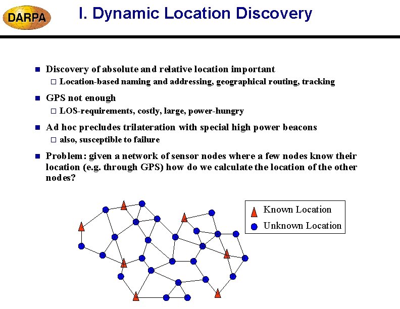
I. Dynamic Location Discovery of absolute and relative location important o n GPS not enough o n LOS-requirements, costly, large, power-hungry Ad hoc precludes trilateration with special high power beacons o n Location-based naming and addressing, geographical routing, tracking also, susceptible to failure Problem: given a network of sensor nodes where a few nodes know their location (e. g. through GPS) how do we calculate the location of the other nodes? Known Location Unknown Location

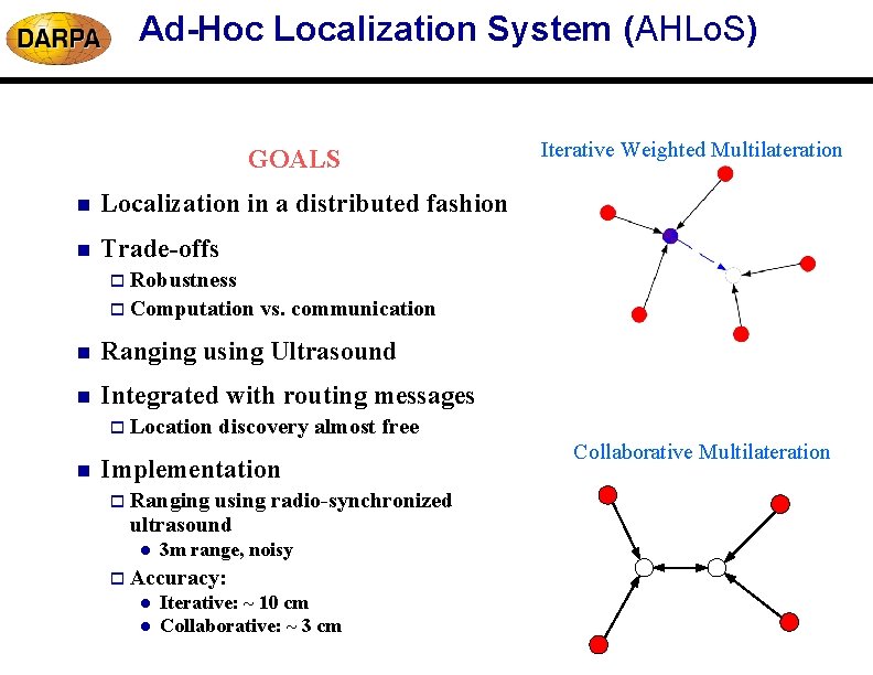
Ad-Hoc Localization System (AHLo. S) GOALS n Localization in a distributed fashion n Trade-offs Iterative Weighted Multilateration o Robustness o Computation vs. communication n Ranging using Ultrasound n Integrated with routing messages o Location n discovery almost free Implementation o Ranging using radio-synchronized ultrasound l 3 m range, noisy o Accuracy: l l Iterative: ~ 10 cm Collaborative: ~ 3 cm Collaborative Multilateration

Iterative Multilateration n Atomic multilateration applied iteratively across the network o may stall if network is sparse, % of beacons is low, terrain obstacles % Resolved Nodes Step 1 Step 3 Step 2 Total Nodes % Initial Beacons Uniformly distributed deployment in a field 100 x 100. Node range = 10.

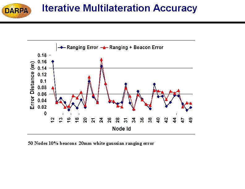
Iterative Multilateration Accuracy 50 Nodes 10% beacons 20 mm white gaussian ranging error

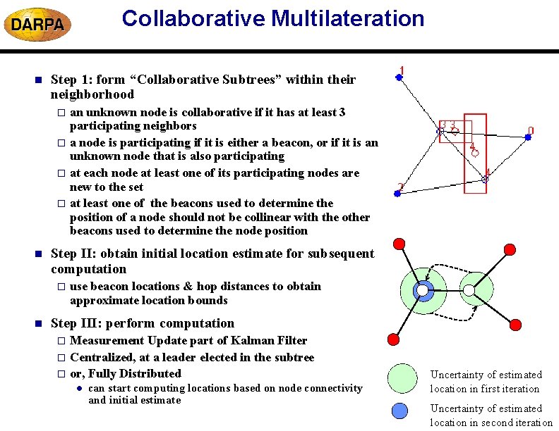
Collaborative Multilateration n Step 1: form “Collaborative Subtrees” within their neighborhood an unknown node is collaborative if it has at least 3 participating neighbors o a node is participating if it is either a beacon, or if it is an unknown node that is also participating o at each node at least one of its participating nodes are new to the set o at least one of the beacons used to determine the position of a node should not be collinear with the other beacons used to determine the node position o n Step II: obtain initial location estimate for subsequent computation o n use beacon locations & hop distances to obtain approximate location bounds Step III: perform computation Measurement Update part of Kalman Filter o Centralized, at a leader elected in the subtree o or, Fully Distributed o l can start computing locations based on node connectivity and initial estimate Uncertainty of estimated location in first iteration Uncertainty of estimated location in second iteration

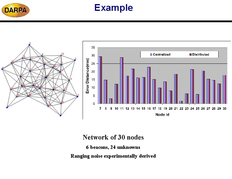
Example Network of 30 nodes 6 beacons, 24 unknowns Ranging noise experimentally derived

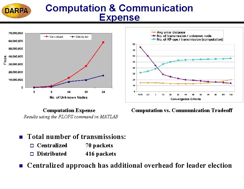
Computation & Communication Expense Computation vs. Communication Tradeoff Results using the FLOPS command in MATLAB n Total number of transmissions: o o n Centralized Distributed 70 packets 416 packets Centralized approach has additional overhead for leader election

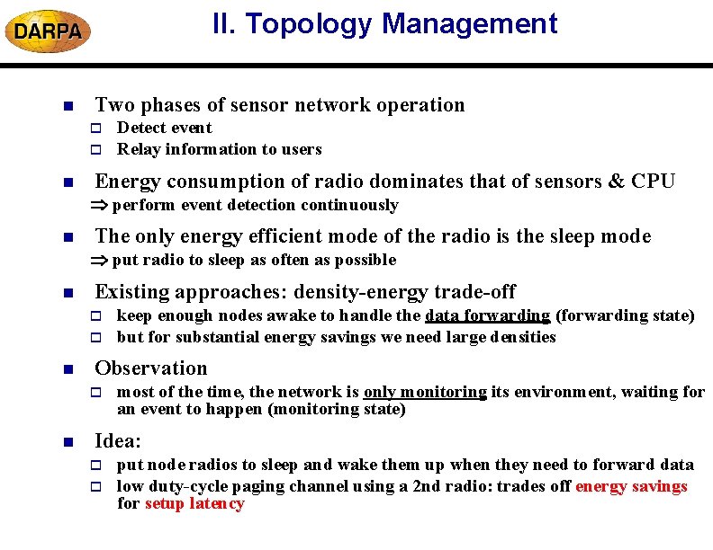
II. Topology Management n Two phases of sensor network operation o o n Detect event Relay information to users Energy consumption of radio dominates that of sensors & CPU perform event detection continuously n The only energy efficient mode of the radio is the sleep mode put radio to sleep as often as possible n Existing approaches: density-energy trade-off o o n Observation o n keep enough nodes awake to handle the data forwarding (forwarding state) but for substantial energy savings we need large densities most of the time, the network is only monitoring its environment, waiting for an event to happen (monitoring state) Idea: o o put node radios to sleep and wake them up when they need to forward data low duty-cycle paging channel using a 2 nd radio: trades off energy savings for setup latency

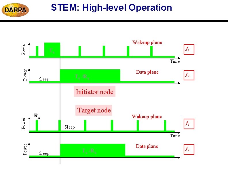
STEM: High-level Operation Power Wakeup plane f 1 Tx Power Time Sleep Tx /Rx Data plane f 2 Power Initiator node Target node Rx Wakeup plane f 1 Sleep Power Time Sleep Tx /Rx Data plane f 2

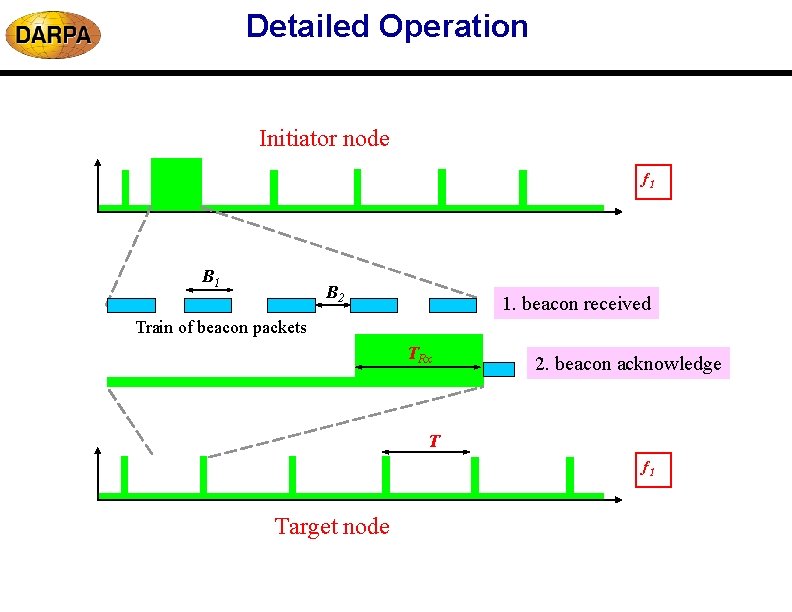
Detailed Operation Initiator node f 1 B 2 1. beacon received Train of beacon packets TRx 2. beacon acknowledge T f 1 Target node

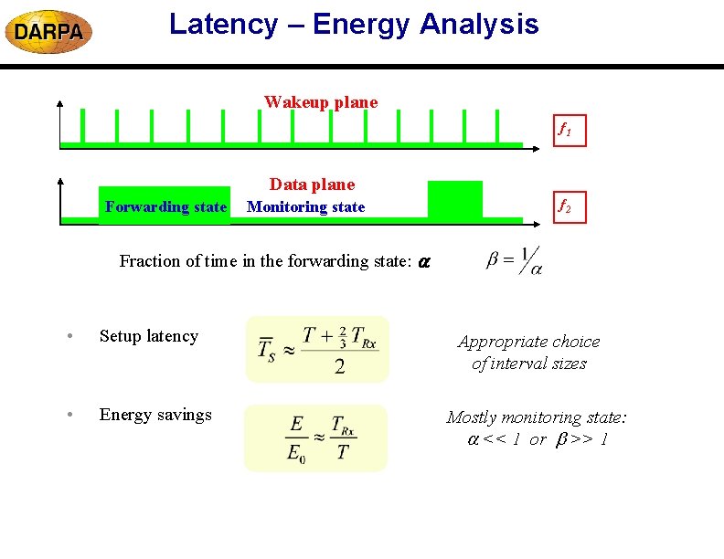
Latency – Energy Analysis Wakeup plane f 1 Data plane Forwarding state Monitoring state f 2 Fraction of time in the forwarding state: • Setup latency • Energy savings Appropriate choice of interval sizes Mostly monitoring state: << 1 or >> 1

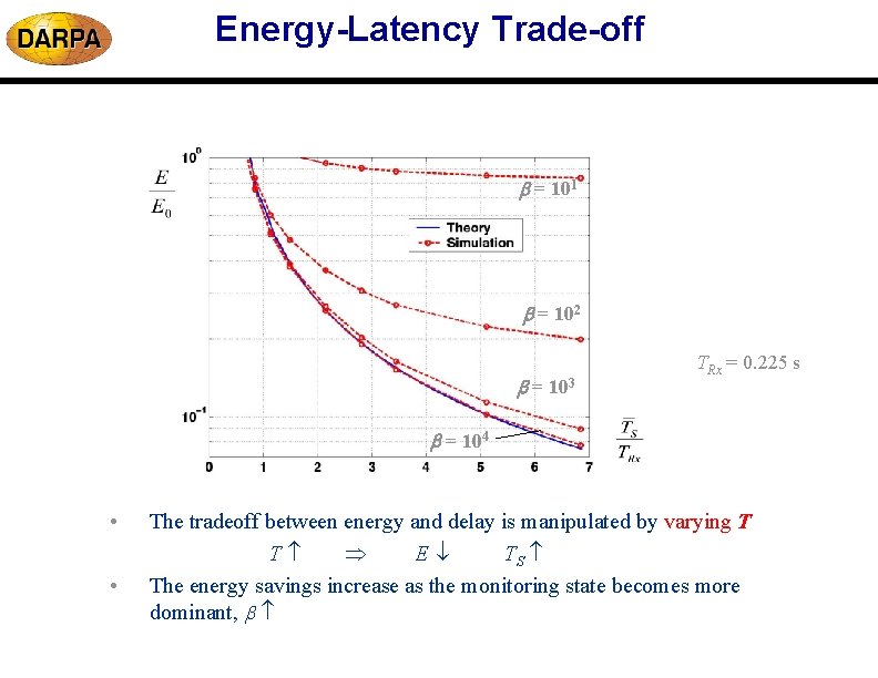
Energy-Latency Trade-off = 101 = 102 = 103 TRx = 0. 225 s = 104 • • The tradeoff between energy and delay is manipulated by varying T T E TS The energy savings increase as the monitoring state becomes more dominant,

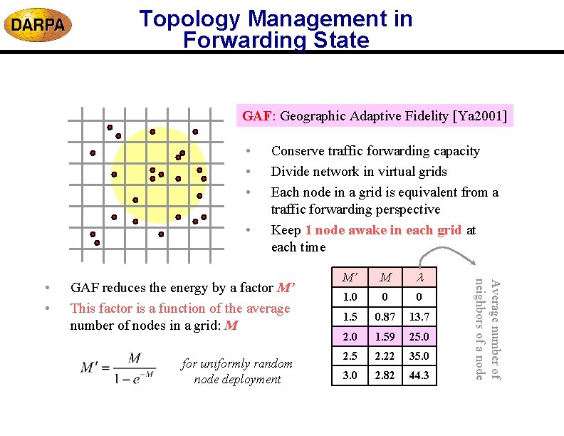
Topology Management in Forwarding State GAF: Geographic Adaptive Fidelity [Ya 2001] • • GAF reduces the energy by a factor M’ This factor is a function of the average number of nodes in a grid: M for uniformly random node deployment M’ M 1. 0 0 0 1. 5 0. 87 13. 7 2. 0 1. 59 25. 0 2. 5 2. 22 35. 0 3. 0 2. 82 44. 3 Average number of neighbors of a node • • Conserve traffic forwarding capacity Divide network in virtual grids Each node in a grid is equivalent from a traffic forwarding perspective Keep 1 node awake in each grid at each time

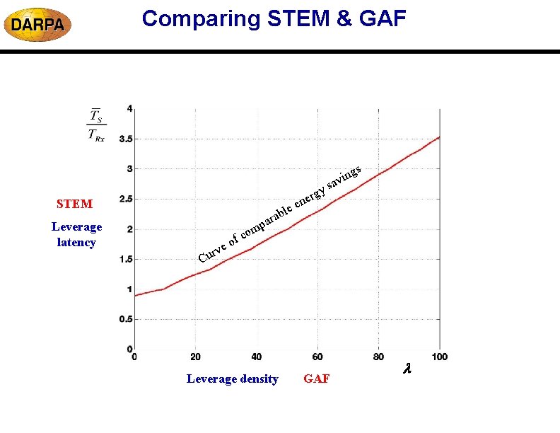
Comparing STEM & GAF gy r e en e l ab STEM Leverage latency gs n i av s ar p m o e rv u C c of Leverage density GAF

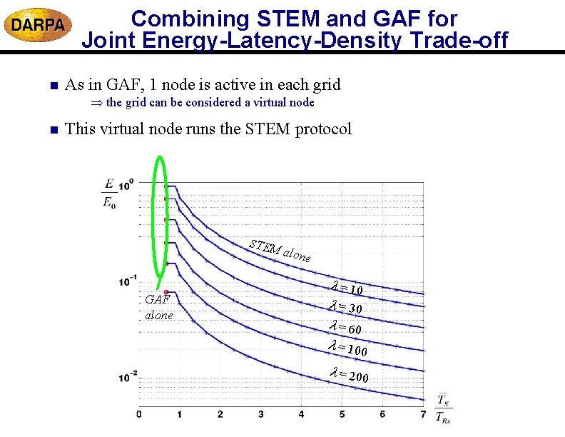
Combining STEM and GAF for Joint Energy-Latency-Density Trade-off n As in GAF, 1 node is active in each grid the grid can be considered a virtual node n This virtual node runs the STEM protocol STEM GAF alone = 10 = 30 = 60 = 100 = 200

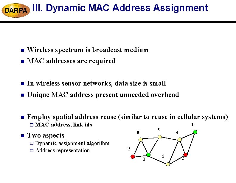
III. Dynamic MAC Address Assignment n Wireless spectrum is broadcast medium n MAC addresses are required n In wireless sensor networks, data size is small n Unique MAC address present unneeded overhead n Employ spatial address reuse (similar to reuse in cellular systems) o MAC n address, link ids 1 Two aspects assignment algorithm o Address representation 5 0 4 o Dynamic 2 1 3 2

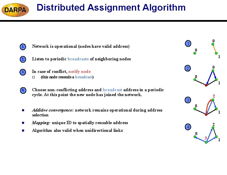
Distributed Assignment Algorithm 1. Network is operational (nodes have valid address) 2. Listen to periodic broadcasts of neighboring nodes 3. In case of conflict, notify node o 0 1 0 2 0 (this node resends a broadcast) 1 4. Choose non-conflicting address and broadcast address in a periodic cycle. At this point the new node has joined the network. 2 3 n Additive convergence: network remains operational during address selection n Mapping: unique ID to spatially reusable address n Algorithm also valid when unidirectional links 0 1 2 4 0 3 1

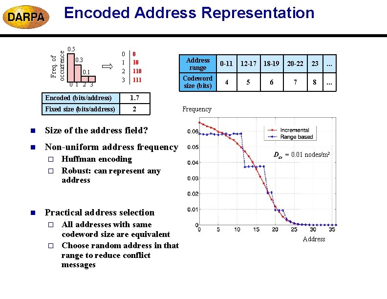
Freq. of occurrence Encoded Address Representation 0. 5 0. 3 0. 1 0 1 2 3 0 1 2 0 10 110 Address range 0 -11 12 -17 18 -19 20 -22 23 … 3 111 Codeword size (bits) 4 5 6 7 8 … Encoded (bits/address) 1. 7 Fixed size (bits/address) 2 n Size of the address field? n Non-uniform address frequency o o n Huffman encoding Robust: can represent any address Frequency Dav = 0. 01 nodes/m 2 Practical address selection o o All addresses with same codeword size are equivalent Choose random address in that range to reduce conflict messages Address

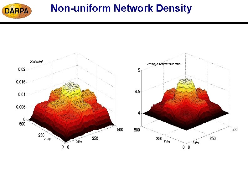
Non-uniform Network Density Nodes/m 2 Average address size (bits) Y (m) X(m)

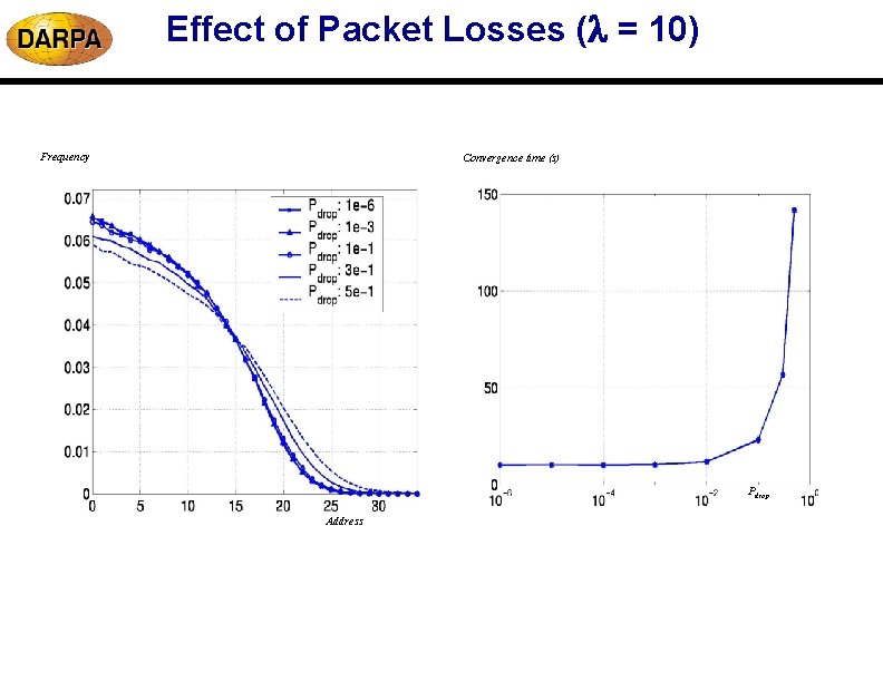
Effect of Packet Losses ( = 10) Frequency Convergence time (s) Pdrop Address

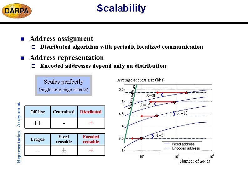
Scalability Address assignment Distributed algorithm with periodic localized communication o n Address representation Encoded addresses depend only on distribution o Average address size (bits) ess Scales perfectly Representation Assignment e addr (neglecting edge effects) Off-line Centralized Distributed ++ - + Unique Fixed reusable Encoded reusable -- + Uniqu n =20 =15 =10 =5 Number of nodes

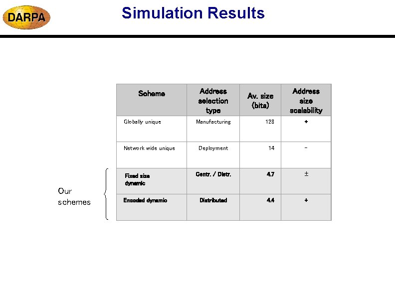
Simulation Results Scheme Globally unique Network wide unique Fixed size dynamic Our schemes Encoded dynamic Address selection type Av. size (bits) Address size scalability Manufacturing 128 + Deployment 14 Centr. / Distr. 4. 7 Distributed 4. 4 +

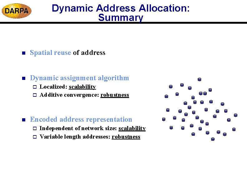
Dynamic Address Allocation: Summary n Spatial reuse of address n Dynamic assignment algorithm o o n Localized: scalability Additive convergence: robustness Encoded address representation o o Independent of network size: scalability Variable length addresses: robustness