Analysis Using SPSS for windows Part I Univariate

Analysis Using SPSS for windows Part I (Univariate and Bivarate) Negussie Deyessa, MD, Ph. D Aug, 2015

When do we do data analysis? • COLLECT DATA: – various methods are used to collect data – (interview, self administered, records, etc) • Data entered to a computer – Use of software (epi-info) • CLEAN/PREPARE DATA: – – Use of simple frequency Tabulation for consistency Ascending and descending Transforming of variables etc • Now it’s time to analyze it! – look for objectives, type of variables & designs, Negussie D, 2012 2

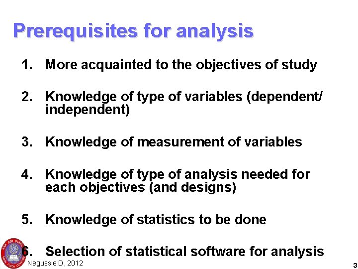
Prerequisites for analysis 1. More acquainted to the objectives of study 2. Knowledge of type of variables (dependent/ independent) 3. Knowledge of measurement of variables 4. Knowledge of type of analysis needed for each objectives (and designs) 5. Knowledge of statistics to be done 6. Selection of statistical software for analysis Negussie D, 2012 3

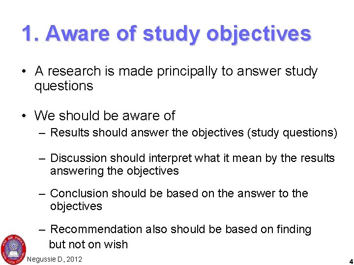
1. Aware of study objectives • A research is made principally to answer study questions • We should be aware of – Results should answer the objectives (study questions) – Discussion should interpret what it mean by the results answering the objectives – Conclusion should be based on the answer to the objectives – Recommendation also should be based on finding but not on wish Negussie D, 2012 4

Cont…. • Results should answer the objectives (study questions) Eg – To determine prevalence of TB in a community – Assess factors associated with HIV/ AIDS – Measure effect of multiple partner on HIV/AIDS prevalence Negussie D, 2012 5

Cont… ♦ Discussion should interpret what it mean by the results answering the objectives Eg – Prevalence of HIV was 10% – Multiple partner was associated with HIV Negussie D, 2012 6

2. Knowledge of type of variables • Knowledge of the dependent and independent variable of the research is important • Knowledge of type of variable the dependent and independent variables are is also needed • What is a variable? Negussie D, 2012 7

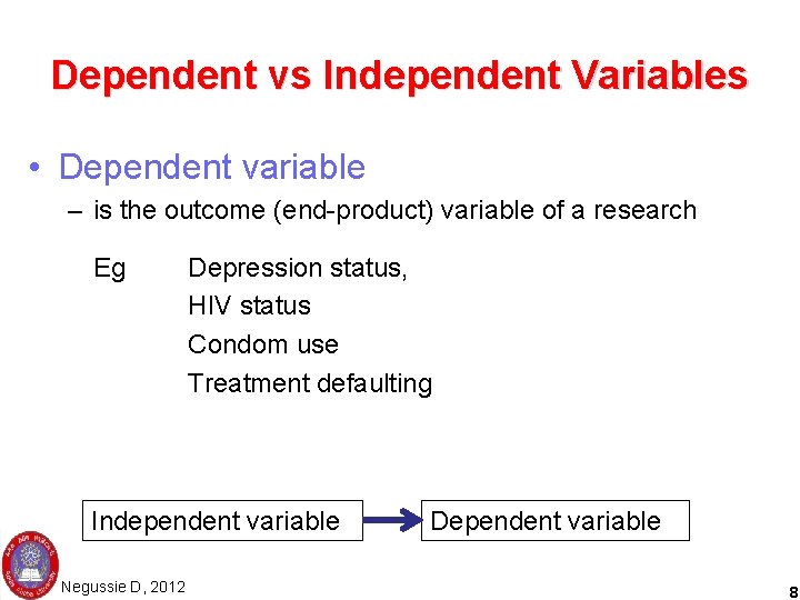
Dependent vs Independent Variables • Dependent variable – is the outcome (end-product) variable of a research Eg Depression status, HIV status Condom use Treatment defaulting Independent variable Negussie D, 2012 Dependent variable 8

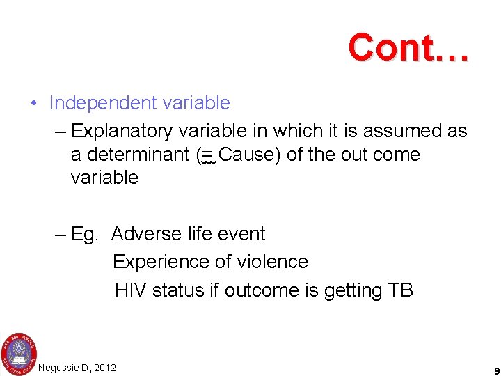
Cont… • Independent variable – Explanatory variable in which it is assumed as a determinant (= Cause) of the out come variable – Eg. Adverse life event Experience of violence HIV status if outcome is getting TB Negussie D, 2012 9

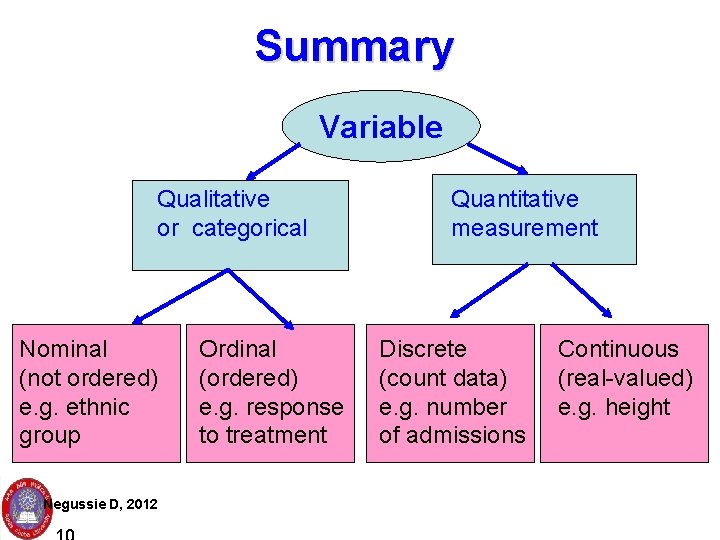
SUMMARY Summary Variable Types of variables Qualitative or categorical Nominal (not ordered) e. g. ethnic group Negussie D, 2012 Ordinal (ordered) e. g. response to treatment Quantitative measurement Discrete (count data) e. g. number of admissions Measurement scales Continuous (real-valued) e. g. height

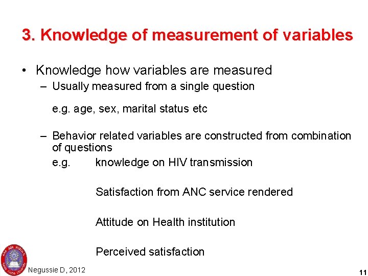
3. Knowledge of measurement of variables • Knowledge how variables are measured – Usually measured from a single question e. g. age, sex, marital status etc – Behavior related variables are constructed from combination of questions e. g. knowledge on HIV transmission Satisfaction from ANC service rendered Attitude on Health institution Perceived satisfaction Negussie D, 2012 11

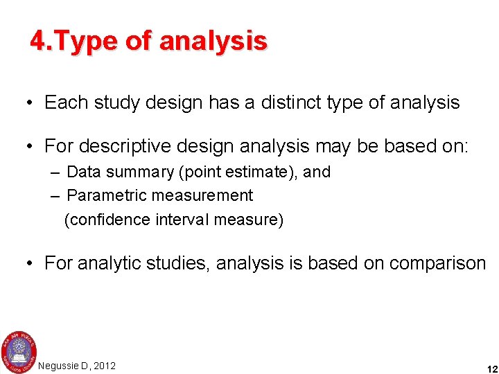
4. Type of analysis • Each study design has a distinct type of analysis • For descriptive design analysis may be based on: – Data summary (point estimate), and – Parametric measurement (confidence interval measure) • For analytic studies, analysis is based on comparison Negussie D, 2012 12

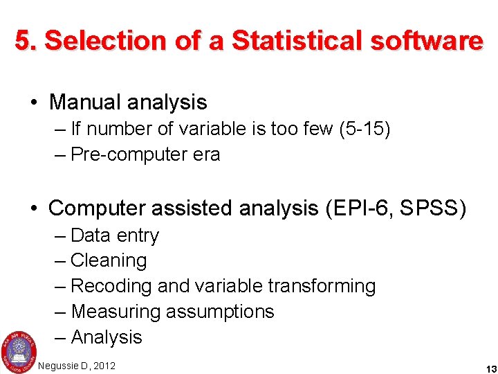
5. Selection of a Statistical software • Manual analysis – If number of variable is too few (5 -15) – Pre-computer era • Computer assisted analysis (EPI-6, SPSS) – Data entry – Cleaning – Recoding and variable transforming – Measuring assumptions – Analysis Negussie D, 2012 13

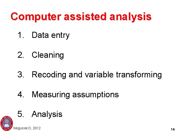
Computer assisted analysis 1. Data entry 2. Cleaning 3. Recoding and variable transforming 4. Measuring assumptions 5. Analysis Negussie D, 2012 14

1. Data entry • It is a process of entering raw data into a computer • It is a process where raw data could be manipulated and changed • Data is coded and entered into a computer Negussie D, 2012 15

2. Data cleaning • Once data is entered, the second step is data cleaning • Data cleaning is a process of similarizing data entered in a computer (soft copy) with that of the hard copy on a paper • Data cleaning goes at three occasions, 1. During template formation 2. During data entry 3. After data is entered (the more we use combination of the above cleaning process, the more accurate will be our data) Negussie D, 2012 16

3. Cleaning after data entry is completed • It is by making a) Simple frequency, b) Tabulating variables for consistency, and c) Sorting • Out layers and missing values are usually evaluated (against hard copy) • Giving serial number for the hard and soft copy makes things simple • Data cleaning by SPSS will be the next session Negussie D, 2012 17

a. Cleaning using simple frequency • By doing simple frequency – You are able to observe values entered to each variable – When you find an option different from your expectation, you should counter check with hard copy – By going to the soft copy, you can check with the hard copy Negussie D, 2012 18

b) Tabulating variables for consistency • This is by cross tabulating one variable against others • If you find variables that will not fit to each other, you can go to reality Eg. Pregnancy Vs. sex Male becoming pregnant Negussie D, 2012 19

c) Cleaning using sorting • When you sort a variable in spreadsheet, you can arrange from – lowest to the highest (ascending) – Highest to the lowest (descending) • Ascending sorting can show you options below your expectation including missing values – This could make you cautious of counter checking to hard copy • Descending sorting can bring numerical numbers above your expectation – You are able to correct or check with hard copy Negussie D, 2012 20

When do we do data analysis? • Next would be: to analyze the data! Negussie D, 2012 21

Three Steps of Data Analysis • Univariate analysis – Step 1: Examine the distribution of each individual variable • Bivariate analysis – Step 2: Describe association between pairs of variables (only two variables) • Multivariate analysis – Step 3: Use a statistical model called Regression (Linear or logistic) to examine the relationship between multiple independent variables & a dependent variable – This is done to gain insight into causal relationships (cause & effect) Negussie D, 2012 22

I. Univariate Analysis

Univariate Analysis • UNIvariate analysis is the process of describing the sample by examining and summarizing the distribution of each individual variable. • Can be used for all variables, regardless of level of measurement • Useful to examine the sample against the source population • It is also useful to make the researcher familiar with variables • It can also be used to test variables for fulfilling assumptions Negussie D, 2012 24

Frequency Distribution • Most basic and usually done for categorical variables • A frequency distribution shows how many cases correspond to each attribute of a variable. • It is like a “tally” or “count” process of a categorical variable. • It also can have proportion (Percent) • Once frequency distribution is done, try to see how it is similar or how it is different from the source population (discussion) Negussie D, 2012 25

Three ways to describe continuous Variables 1. Central tendency – Most common values for a continuous variable 2. Variability (Dispersion) – How cases are distributed across a set of attributes of a variable 3. Shape of the overall distribution (symmetry) Negussie D, 2012 26

Mean for Nominal Variables (special interpretation) • It is the proportion of the sample in the “ 1” category. • Note: You can convert the proportion to a percentage by multiplying by 10 n. Negussie D, 2012 27

Univariate analysis using SPSS for windows

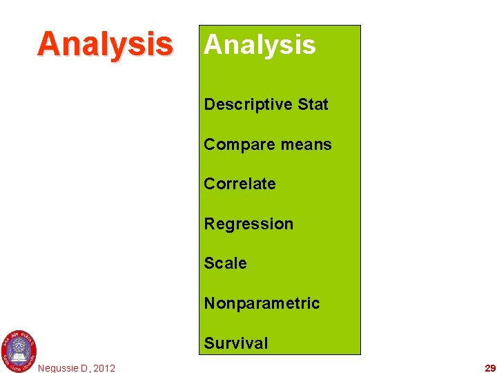
Analysis Descriptive Stat Compare means Correlate Regression Scale Nonparametric Survival Negussie D, 2012 29

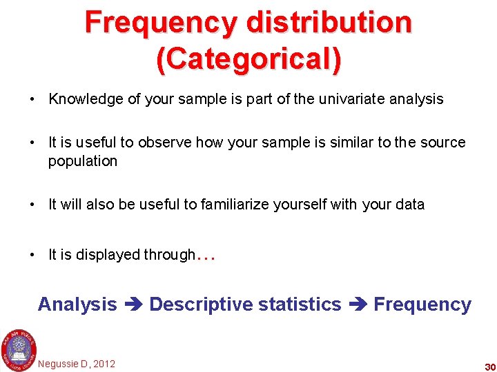
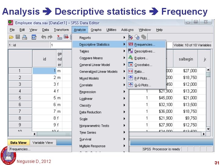
Frequency distribution (Categorical) • Knowledge of your sample is part of the univariate analysis • It is useful to observe how your sample is similar to the source population • It will also be useful to familiarize yourself with your data • It is displayed through… Analysis Descriptive statistics Frequency Negussie D, 2012 30

Analysis Descriptive statistics Frequency Negussie D, 2012 31

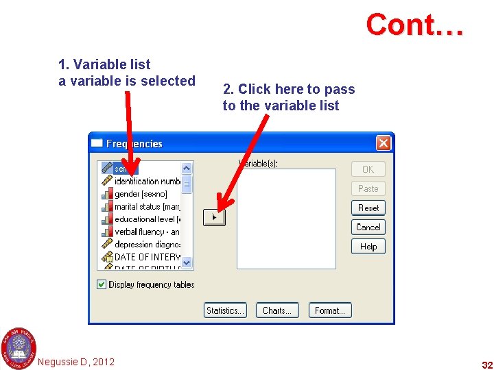
Cont… 1. Variable list a variable is selected Negussie D, 2012 2. Click here to pass to the variable list 32

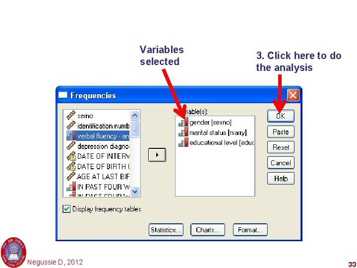
Variables selected Negussie D, 2012 3. Click here to do the analysis 33

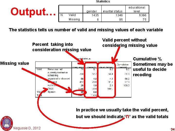
Output…. The statistics tells us number of valid and missing values of each variable Percent taking into consideration missing value Missing value Valid percent without considering missing value Cumulative % Sometimes may be useful to decide recoding In practice we usually take the valid percent, but we should indicate ‘n’ as the valid totals Negussie D, 2012 34

Continuous variables Looking for Assumptions • In SPSS, like any statistical analysis, it goes through lots of assumptions • Dependent and continuous variables should go through these assumptions • These continuous variables should be tested for their symmetrical distribution • If not, they should not pass through many methods of analysis (they should follow non-parametric analysis) • There are two ways to assess summary analysis of a continuous variable Negussie D, 2012 35

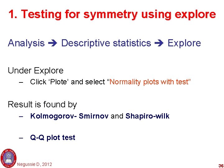
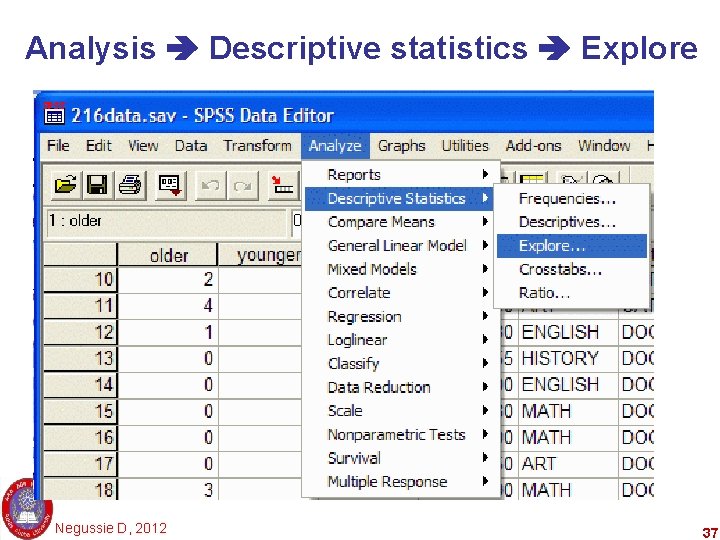
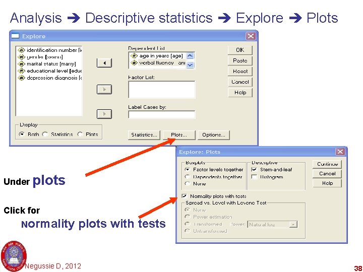
1. Testing for symmetry using explore Analysis Descriptive statistics Explore Under Explore – Click ‘Plote’ and select “Normality plots with test” Result is found by – Kolmogorov- Smirnov and Shapiro-wilk – Q-Q plot test Negussie D, 2012 36

Analysis Descriptive statistics Explore Negussie D, 2012 37

Analysis Descriptive statistics Explore Plots Under plots Click for Normality plots with tests Negussie D, 2012 38

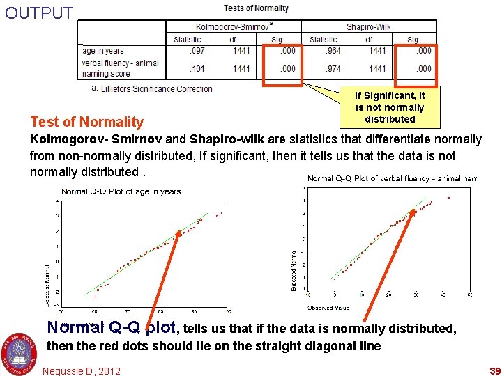
OUTPUT Test of Normality If Significant, it is not normally distributed Kolmogorov- Smirnov and Shapiro-wilk are statistics that differentiate normally from non-normally distributed, If significant, then it tells us that the data is not normally distributed. Normal Q-Q plot, tells us that if the data is normally distributed, then the red dots should lie on the straight diagonal line Negussie D, 2012 39

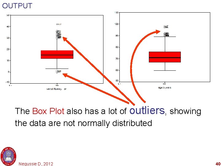
OUTPUT The Box Plot also has a lot of outliers, showing the data are not normally distributed Negussie D, 2012 40

II Bivariate Analysis

Bivariate Analysis • Bivariate analysis is second step in analysis 1. It is analysis made to test presence of relationship between two variables 2. It also could assess presence of difference between two variables. • Answers the question: Is there a relationship or difference between the two variables? • It is initial step in hypothesis testing Negussie D, 2012 42

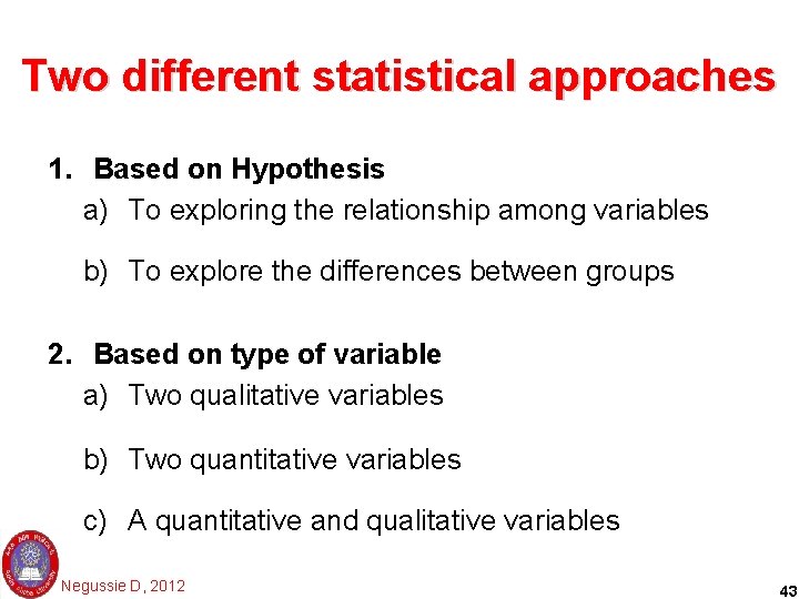
Two different statistical approaches 1. Based on Hypothesis a) To exploring the relationship among variables b) To explore the differences between groups 2. Based on type of variable a) Two qualitative variables b) Two quantitative variables c) A quantitative and qualitative variables Negussie D, 2012 43

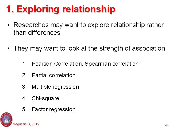
1. Exploring relationship • Researches may want to explore relationship rather than differences • They may want to look at the strength of association 1. Pearson Correlation, Spearman correlation 2. Partial correlation 3. Multiple regression 4. Chi-square 5. Factor regression Negussie D, 2012 44

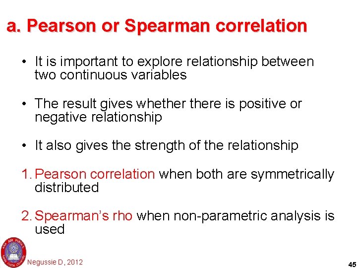
a. Pearson or Spearman correlation • It is important to explore relationship between two continuous variables • The result gives whethere is positive or negative relationship • It also gives the strength of the relationship 1. Pearson correlation when both are symmetrically distributed 2. Spearman’s rho when non-parametric analysis is used Negussie D, 2012 45

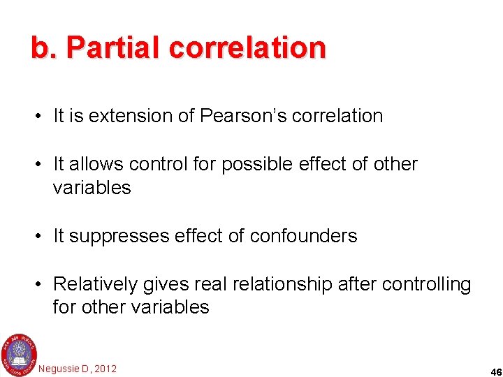
b. Partial correlation • It is extension of Pearson’s correlation • It allows control for possible effect of other variables • It suppresses effect of confounders • Relatively gives real relationship after controlling for other variables Negussie D, 2012 46

c. Multiple regression • More sophisticated extension of correlation • It is used to explore predictive ability of many independent variables on one continuous variable • Different types of multiple regression allow to compare the predictive ability of independent variables to find the best set of variables Negussie D, 2012 47

d. Chi square • It is a statistics that explores relationship between two categorical variables • If the dependent variable is dichotomies the relationship can be expressed on RR or OR • RR for prospective cohort or experimental design while OR for case control or cross sectional design Negussie D, 2012 48

e. Factor analysis • Allows to condense a large set of variables down to a smaller (manageable) dimensions. • It does so through summarizing using pattern of correlation. • Through looking at correlation between variables, it groups the related once. Negussie D, 2012 49

2. Explore differences • It assess significance difference among groups • Suitable when continuous variables with normal distribution 1. T-tests 2. One-way Analysis of Variance (ANOVA) 3. Two-way analysis of Variance 4. Multivariate analysis of variance (MANOVA) 5. Analysis of covariance (ANCOVA) Negussie D, 2012 50

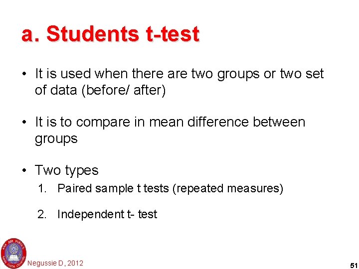
a. Students t-test • It is used when there are two groups or two set of data (before/ after) • It is to compare in mean difference between groups • Two types 1. Paired sample t tests (repeated measures) 2. Independent t- test Negussie D, 2012 51

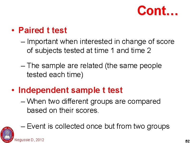
Cont… • Paired t test – Important when interested in change of score of subjects tested at time 1 and time 2 – The sample are related (the same people tested each time) • Independent sample t test – When two different groups are compared based on their scores. – Event is collected once but from two groups Negussie D, 2012 52

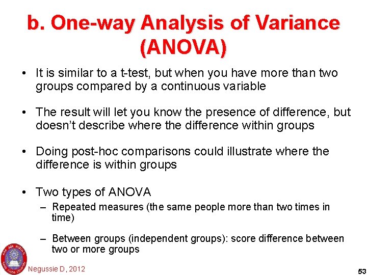
b. One-way Analysis of Variance (ANOVA) • It is similar to a t-test, but when you have more than two groups compared by a continuous variable • The result will let you know the presence of difference, but doesn’t describe where the difference within groups • Doing post-hoc comparisons could illustrate where the difference is within groups • Two types of ANOVA – Repeated measures (the same people more than two times in time) – Between groups (independent groups): score difference between two or more groups Negussie D, 2012 53

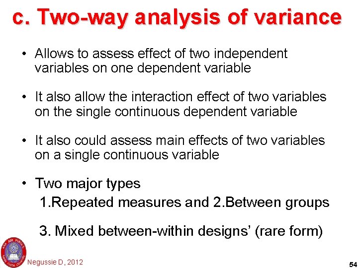
c. Two-way analysis of variance • Allows to assess effect of two independent variables on one dependent variable • It also allow the interaction effect of two variables on the single continuous dependent variable • It also could assess main effects of two variables on a single continuous variable • Two major types 1. Repeated measures and 2. Between groups 3. Mixed between-within designs’ (rare form) Negussie D, 2012 54

d. Multivariate analysis of Variance (MANOVA) • It is used when you want to compare groups on a number (2 -3) similar continuous dependent variables • Example to see the effect of different treatments on variety of outcome measures (eg anxiety, depression, physical symptoms ‘all continuous var. ’) • More sophisticated form of analysis Negussie D, 2012 55

E. Analysis of Covariance (ANCOVA) • Used when you want to statistically control the effect of a third variable (confounder) • It is used when you suspected the third variable could confound (covariate) the difference Negussie D, 2012 56

2. Based on possible combination • There are three possible combination pairs of variable types, • Combination between: 1. Two qualitative variables 2. Two quantitative variables 3. A quantitative and qualitative variables Negussie D, 2012 57

1. Two qualitative variables • This is when the dependent and the independent variables are categorical • The statistics can be done – Manually, – Statcalc of EPI-info, – Crosstab and logistic regression in SPSS. • Chi square is the usual test of statistics Negussie D, 2012 58

1. Two qualitative variables • This is when the dependent and the independent variables are categorical • The statistics can be done – Manually, – Statcalc of EPI-info, – Crosstab and logistic regression in SPSS. • Chi square is the usual test of statistics Negussie D, 2012 59

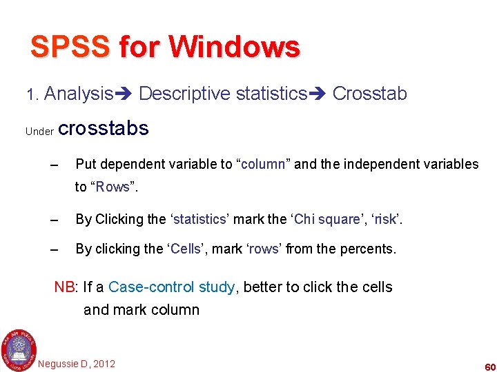
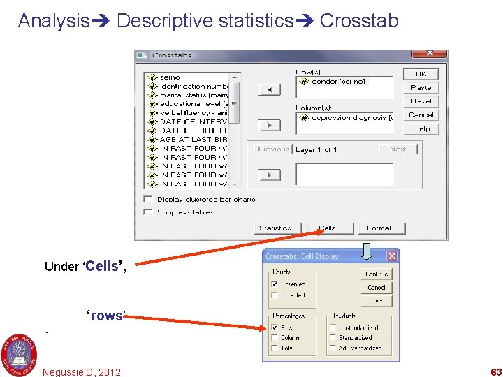
SPSS for Windows 1. Analysis Descriptive statistics Crosstab Under crosstabs – Put dependent variable to “column” and the independent variables to “Rows”. – By Clicking the ‘statistics’ mark the ‘Chi square’, ‘risk’. – By clicking the ‘Cells’, mark ‘rows’ from the percents. NB: If a Case-control study, better to click the cells and mark column Negussie D, 2012 60

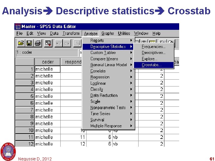
Analysis Descriptive statistics Crosstab Negussie D, 2012 61

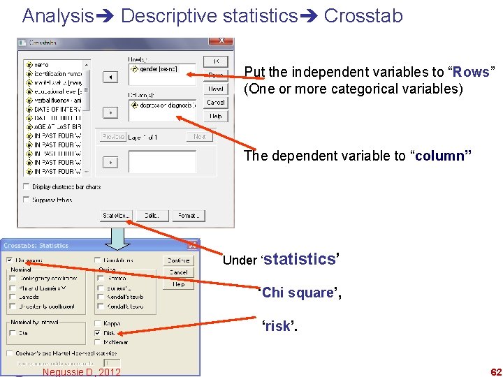
Analysis Descriptive statistics Crosstab Put the independent variables to “Rows” (One or more categorical variables) The dependent variable to “column” Under ‘statistics’ ‘Chi square’, ‘risk’. Negussie D, 2012 62

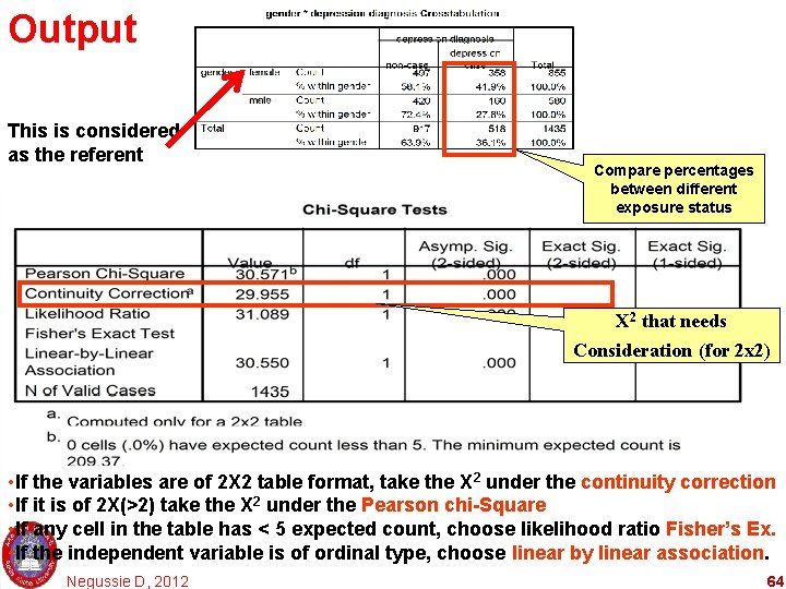
Analysis Descriptive statistics Crosstab Under ‘Cells’, . ‘rows’ Negussie D, 2012 63

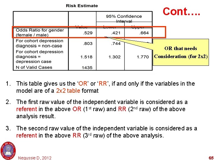
Output This is considered as the referent Compare percentages between different exposure status X 2 that needs Consideration (for 2 x 2) • If the variables are of 2 X 2 table format, take the X 2 under the continuity correction • If it is of 2 X(>2) take the X 2 under the Pearson chi-Square • If any cell in the table has < 5 expected count, choose likelihood ratio Fisher’s Ex. • If the independent variable is of ordinal type, choose linear by linear association. Negussie D, 2012 64

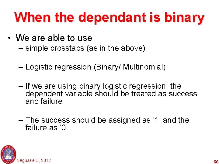
Cont…. OR that needs Consideration (for 2 x 2) 1. This table gives us the ‘OR’ or ‘RR’, if and only if the variables in the model are of a 2 x 2 table format 2. The first raw value of the independent variable is considered as a referent in the above OR (1 st raw) and RR (2 nd raw) of the above analysis result. 3. The second raw value of the independent variable is considered as a referent in the above RR (3 rd raw) of the above analysis. Negussie D, 2012 65

When the dependant is binary • We are able to use – simple crosstabs (as in the above) – Logistic regression (Binary/ Multinomial) – If we are using binary logistic regression, the dependent variable should be treated as success and failure – The success should be assigned as ‘ 1’ and the failure as ‘ 0’ Negussie D, 2012 66

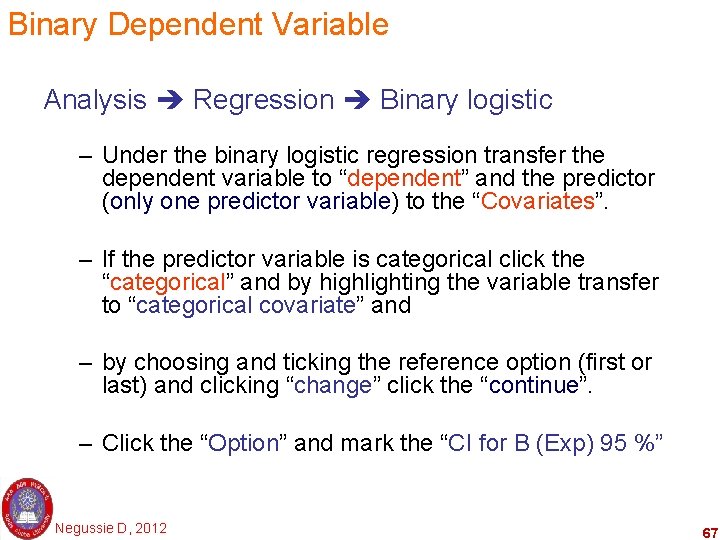
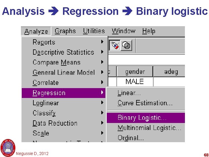
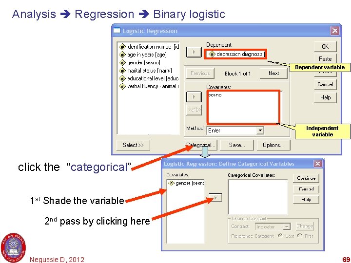
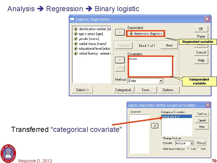
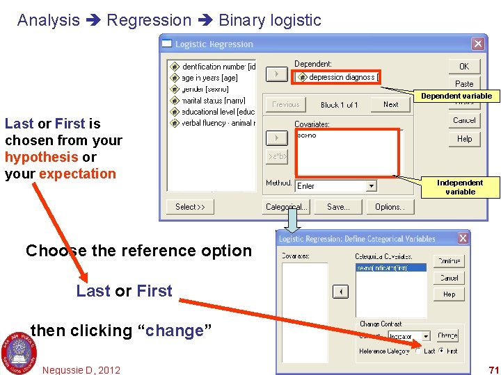
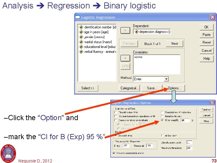
Binary Dependent Variable Analysis Regression Binary logistic – Under the binary logistic regression transfer the dependent variable to “dependent” and the predictor (only one predictor variable) to the “Covariates”. – If the predictor variable is categorical click the “categorical” and by highlighting the variable transfer to “categorical covariate” and – by choosing and ticking the reference option (first or last) and clicking “change” click the “continue”. – Click the “Option” and mark the “CI for B (Exp) 95 %” Negussie D, 2012 67

Analysis Regression Binary logistic Negussie D, 2012 68

Analysis Regression Binary logistic Dependent variable Independent variable click the “categorical” 1 st Shade the variable 2 nd pass by clicking here Negussie D, 2012 69

Analysis Regression Binary logistic Dependent variable Independent variable Transferred “categorical covariate” Negussie D, 2012 70

Analysis Regression Binary logistic Dependent variable Last or First is chosen from your hypothesis or your expectation Independent variable Choose the reference option Last or First then clicking “change” Negussie D, 2012 71

Choosing the referent [NB] • One or more values of the independent variable is considered as exposure and non-exposure variable • The referent of the independent variable is selected by our hypothesis, experience or changeability of natural occurrence • Usually normal occurrence is considered as referent (nonexposure) • This postulated reference should be arranged (ordered) as First or Last. • We then have to choose this referent according to its place in order of its existence Negussie D, 2012 72

Analysis Regression Binary logistic –Click the “Option” and –mark the “CI for B (Exp) 95 %” Negussie D, 2012 73

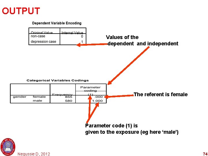
OUTPUT Values of the dependent and independent The referent is female Parameter code (1) is given to the exposure (eg here ‘male’) Negussie D, 2012 74

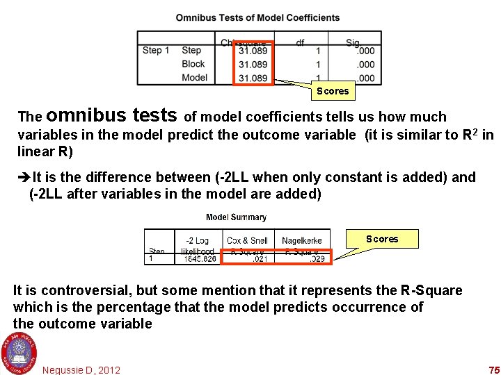
Scores The omnibus tests of model coefficients tells us how much variables in the model predict the outcome variable (it is similar to R 2 in linear R) It is the difference between (-2 LL when only constant is added) and (-2 LL after variables in the model are added) Scores It is controversial, but some mention that it represents the R-Square which is the percentage that the model predicts occurrence of the outcome variable Negussie D, 2012 75

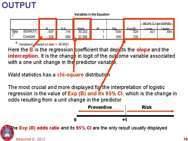
OUTPUT Here the B is the regression coefficient that depicts the slope and the interception. It is the change in logit of the outcome variable associated with a one unit change in the predictor variable. Wald statistics has a chi-square distribution The most crucial and more displayed for the interpretation of logistic regression is the value of Exp (B) and its 95% CI, which is the change in odds resulting from a unit change in the predictor Preventive 0 Risk +1 The Exp (B) odds ratio and its 95% CI are the only result usually displayed Negussie D, 2012 76

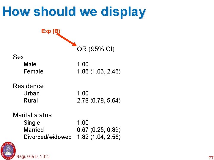
How should we display Exp (B) OR (95% CI) Sex Male Female 1. 00 1. 86 (1. 05, 2. 46) Residence Urban Rural 1. 00 2. 78 (0. 78, 5. 64) Marital status Single 1. 00 Married 0. 67 (0. 25, 0. 89) Divorced/widowed 1. 82 (1. 04, 2. 56) Negussie D, 2012 77

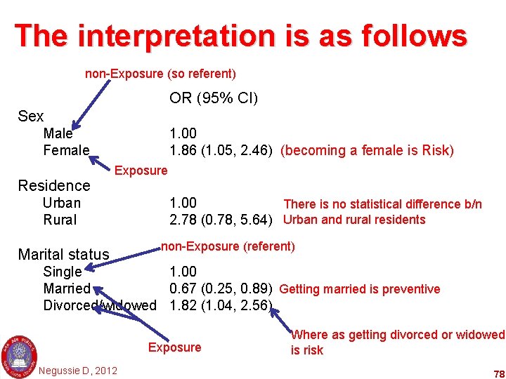
The interpretation is as follows non-Exposure (so referent) OR (95% CI) Sex Male Female Residence 1. 00 1. 86 (1. 05, 2. 46) (becoming a female is Risk) Exposure Urban Rural Marital status 1. 00 There is no statistical difference b/n 2. 78 (0. 78, 5. 64) Urban and rural residents non-Exposure (referent) Single 1. 00 Married 0. 67 (0. 25, 0. 89) Getting married is preventive Divorced/widowed 1. 82 (1. 04, 2. 56) Exposure Negussie D, 2012 Where as getting divorced or widowed is risk 78

2. Two quantitative variables • Uses a correlation matrix • Pearson’s correlation is used, when the two variables – are continuous and – are symmetrically distributed • Therefore, we should test the variables for their symmetry • If they fulfill for symmetry, we are able to analyze using the Pearson’s correlation matrix Negussie D, 2012 79

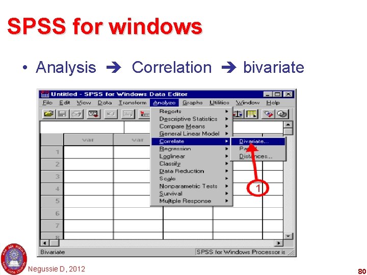
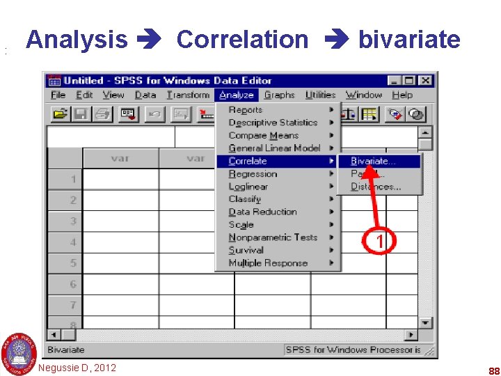
SPSS for windows • Analysis Correlation bivariate Negussie D, 2012 80

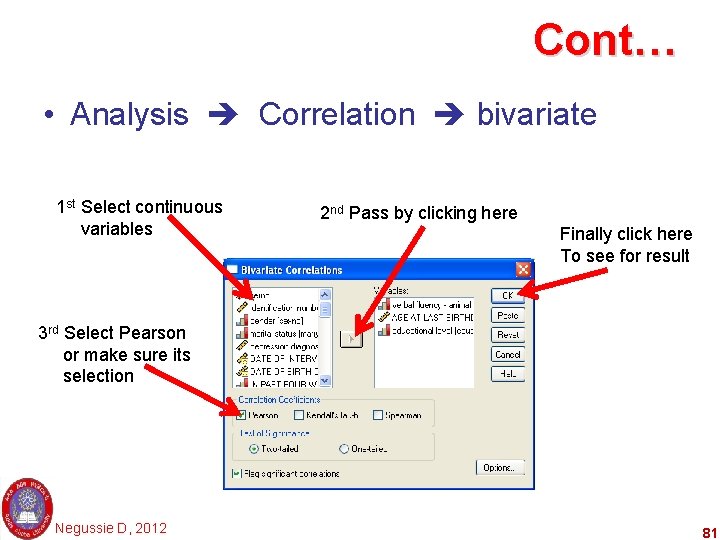
Cont… • Analysis Correlation bivariate 1 st Select continuous variables 2 nd Pass by clicking here Finally click here To see for result 3 rd Select Pearson or make sure its selection Negussie D, 2012 81

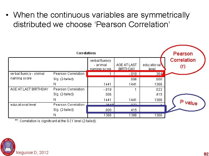
• When the continuous variables are symmetrically distributed we choose ‘Pearson Correlation’ Pearson Correlation (r) P value Negussie D, 2012 82

The result of analysis • Pearson’s Correlation Coefficient (r) – Tells you two things about the relationship: 1. Strength? 2. Direction? – Also, the p-value: 3. Significant? Negussie D, 2012 83

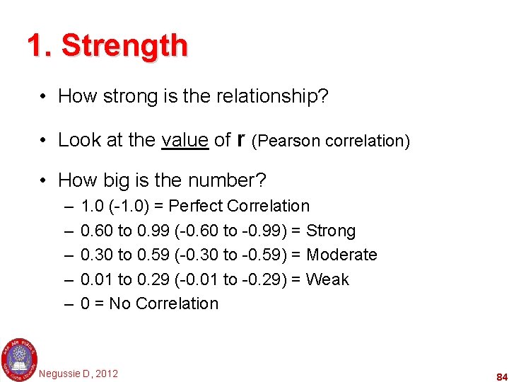
1. Strength • How strong is the relationship? • Look at the value of r (Pearson correlation) • How big is the number? – – – 1. 0 (-1. 0) = Perfect Correlation 0. 60 to 0. 99 (-0. 60 to -0. 99) = Strong 0. 30 to 0. 59 (-0. 30 to -0. 59) = Moderate 0. 01 to 0. 29 (-0. 01 to -0. 29) = Weak 0 = No Correlation Negussie D, 2012 84

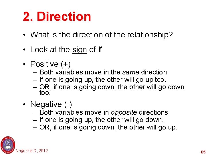
2. Direction • What is the direction of the relationship? • Look at the sign of r • Positive (+) – Both variables move in the same direction – If one is going up, the other will go up too. – OR, if one is going down, the other will go down too. • Negative (-) – Both variables move in opposite directions – If one is going up, the other will go down. – OR, if one is going down, the other will go up. Negussie D, 2012 85

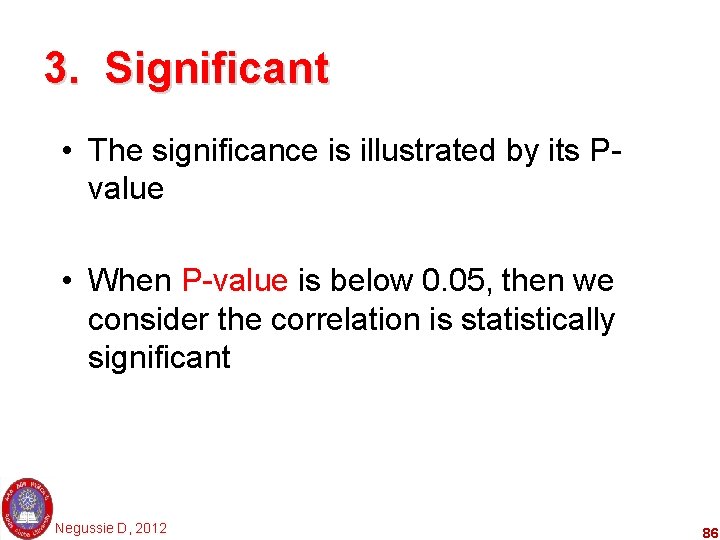
3. Significant • The significance is illustrated by its Pvalue • When P-value is below 0. 05, then we consider the correlation is statistically significant Negussie D, 2012 86

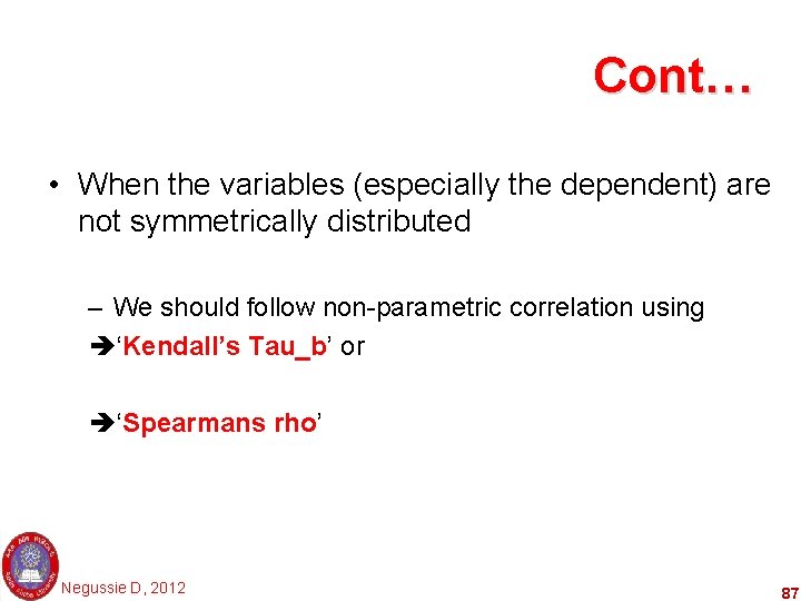
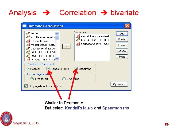
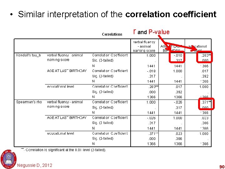
Cont… • When the variables (especially the dependent) are not symmetrically distributed – We should follow non-parametric correlation using ‘Kendall’s Tau_b’ or ‘Spearmans rho’ Negussie D, 2012 87

: Analysis Correlation bivariate Negussie D, 2012 88

Analysis Correlation bivariate Similar to Pearson c. But select Kendall’s tau-b and Spearman rho Negussie D, 2012 89

• Similar interpretation of the correlation coefficient r and P-value Negussie D, 2012 90

3. A qualitative & a quantitative variable • Here you can look at a difference in mean values between two or more groups • Statistics of significance is made by: – ‘Students t-test” for two groups, and – ‘F-test’ for more than two groups • P-value is seen to judge for significance – P < 0. 05, it is significant – P > 0. 05, it is NOT significant Negussie D, 2012 91

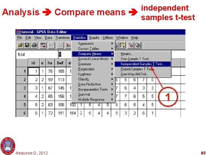
SPSS for windows • If the dependent variable is symmetrically distributed, look for the independent variable 1. If it is categorical and binary type, Use ‘students t-test’. independent Analysis Compare means samples t-test Negussie D, 2012 92

independent Analysis Compare means samples t-test : Negussie D, 2012 93

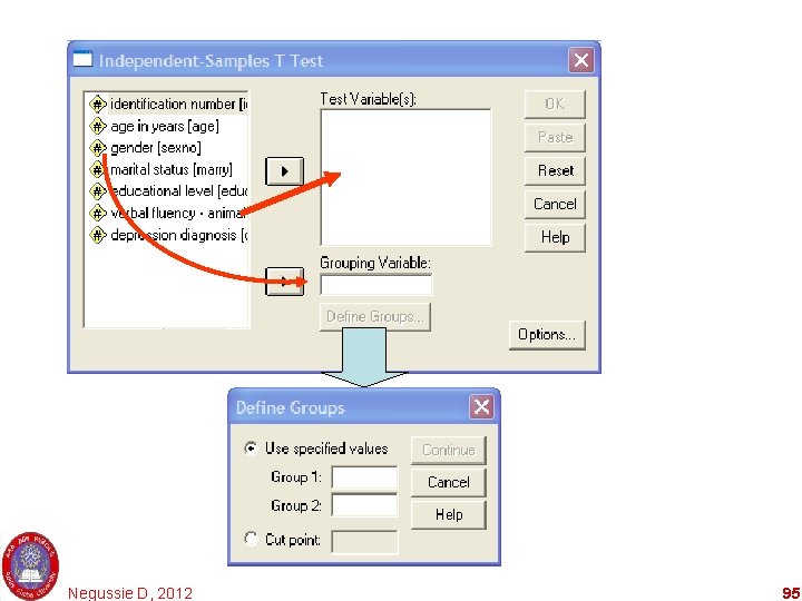
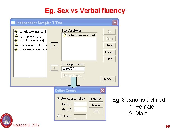
Within independent samples t-test…. . • Select the dependent variable to the ‘test variable’ space and the independent variable to the ‘grouping variables’. • Define the independent variable as their labeled number, and click the ‘Ok’. • This will give you the mean difference and its significance using t-test. Negussie D, 2012 94

Negussie D, 2012 95

Eg. Sex vs Verbal fluency Eg ‘Sexno’ is defined 1. Female 2. Male Negussie D, 2012 96

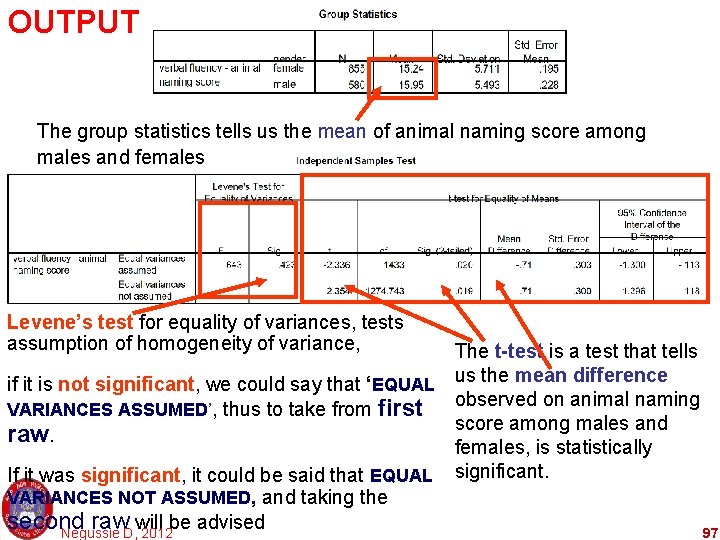
OUTPUT The group statistics tells us the mean of animal naming score among males and females Levene’s test for equality of variances, tests assumption of homogeneity of variance, if it is not significant, we could say that ‘EQUAL VARIANCES ASSUMED’, thus to take from first raw. If it was significant, it could be said that EQUAL VARIANCES NOT ASSUMED, and taking the second raw will be advised Negussie D, 2012 The t-test is a test that tells us the mean difference observed on animal naming score among males and females, is statistically significant. 97

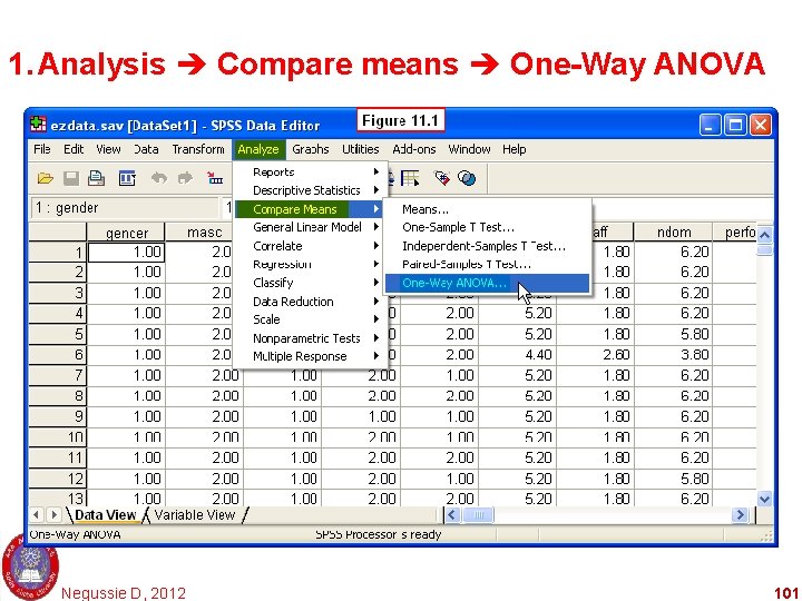
SPSS for windows • If the dependent variable is symmetrically distributed, look for the independent variable 2. If it is categorical and non-binary type, Use F-test. 1. Analysis Compare means One-Way ANOVA 2. Analysis Regression Linear Negussie D, 2012 98

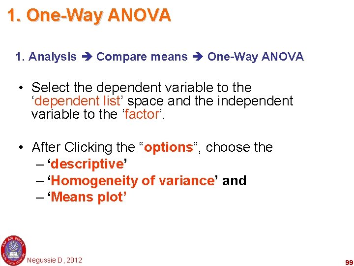
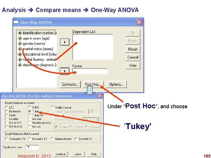
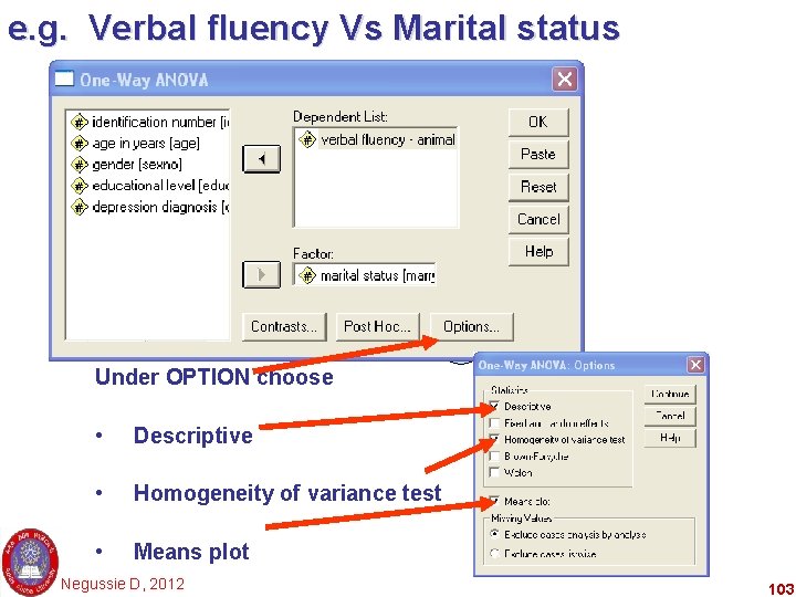
1. One-Way ANOVA 1. Analysis Compare means One-Way ANOVA • Select the dependent variable to the ‘dependent list’ space and the independent variable to the ‘factor’. • After Clicking the “options”, choose the – ‘descriptive’ – ‘Homogeneity of variance’ and – ‘Means plot’ Negussie D, 2012 99

Cont… • After clicking “Post Hoc”, choose ‘Tukey’, click the ‘Ok’. – This will give you the mean difference between and within group difference and its significance using F-test. – It also gives you Regression coefficients (the intercept and the slop) Negussie D, 2012 100

1. Analysis Compare means One-Way ANOVA Negussie D, 2012 101

Analysis Compare means One-Way ANOVA Under “Post Hoc”, and choose ‘Tukey’ Negussie D, 2012 102

e. g. Verbal fluency Vs Marital status Under OPTION choose • Descriptive • Homogeneity of variance test • Means plot Negussie D, 2012 103

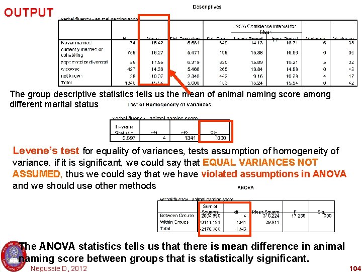
OUTPUT The group descriptive statistics tells us the mean of animal naming score among different marital status Levene’s test for equality of variances, tests assumption of homogeneity of variance, if it is significant, we could say that EQUAL VARIANCES NOT ASSUMED, thus we could say that we have violated assumptions in ANOVA and we should use other methods The ANOVA statistics tells us that there is mean difference in animal naming score between groups that is statistically significant. Negussie D, 2012 104

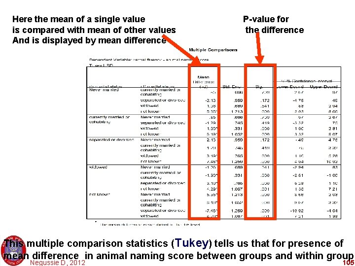
Here the mean of a single value is compared with mean of other values And is displayed by mean difference P-value for the difference This multiple comparison statistics (Tukey) tells us that for presence of mean difference in animal naming score between groups and within groups Negussie D, 2012 105

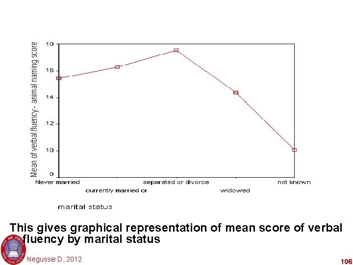
This gives graphical representation of mean score of verbal fluency by marital status Negussie D, 2012 106

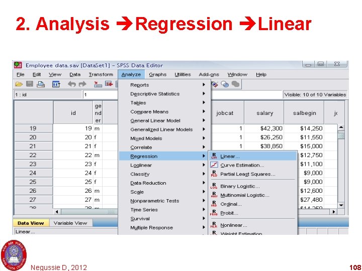
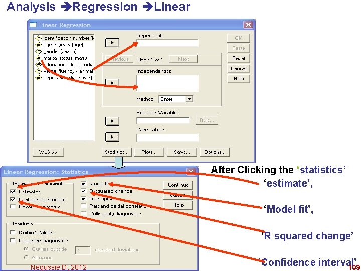
2. Analysis Regression Linear • Select the dependent variable to the ‘dependent’ space and the independent variable to the ‘independent’. • After Clicking the ‘statistics’, chose the ‘estimate’, ‘model fit’, ‘confidence interval’ and ‘R squared change’ and click the ‘Ok’. – This will give you the mean difference between and within group difference and its significance is measured using F-test. – It also gives you regression coefficients (the intercept and the slop) – (the ß = slop , gives you positive or negative relationship between the predictor and the Outcome Variable) – It also gives you R 2 which is the explanatory or prediction power of the model in predicting the outcome variable. Negussie D, 2012 107

2. Analysis Regression Linear Negussie D, 2012 108

Analysis Regression Linear After Clicking the ‘statistics’ ‘estimate’, ‘Model fit’, ‘R squared change’ Negussie D, 2012 ‘Confidence interval’ 109

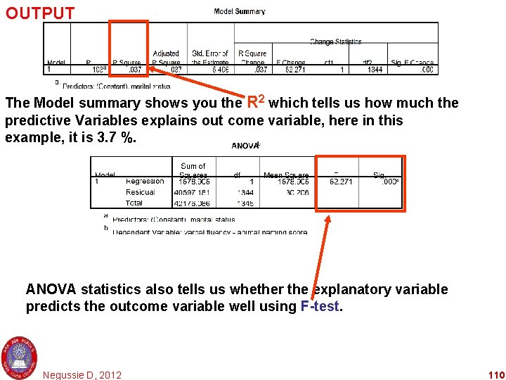
OUTPUT The Model summary shows you the R 2 which tells us how much the predictive Variables explains out come variable, here in this example, it is 3. 7 %. ANOVA statistics also tells us whether the explanatory variable predicts the outcome variable well using F-test. Negussie D, 2012 110

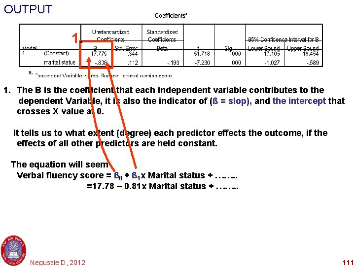
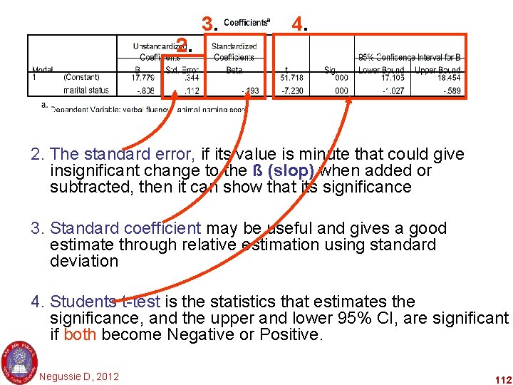
OUTPUT 1. The B is the coefficient that each independent variable contributes to the dependent Variable, it is also the indicator of (ß = slop), and the intercept that crosses X value at 0. It tells us to what extent (degree) each predictor effects the outcome, if the effects of all other predictors are held constant. The equation will seem Verbal fluency score = ß 0 + ß 1 x Marital status + ……. . =17. 78 – 0. 81 x Marital status + ……. . Negussie D, 2012 111

2. 3. 4. 2. The standard error, if its value is minute that could give insignificant change to the ß (slop) when added or subtracted, then it can show that its significance 3. Standard coefficient may be useful and gives a good estimate through relative estimation using standard deviation 4. Students t-test is the statistics that estimates the significance, and the upper and lower 95% CI, are significant if both become Negative or Positive. Negussie D, 2012 112

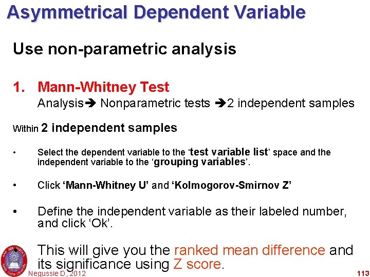
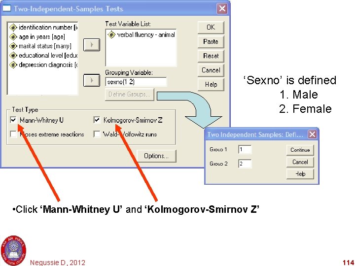
Asymmetrical Dependent Variable Use non-parametric analysis 1. Mann-Whitney Test Analysis Nonparametric tests 2 independent samples Within 2 independent samples • Select the dependent variable to the ‘test variable list’ space and the independent variable to the ‘grouping variables’. • Click ‘Mann-Whitney U’ and ‘Kolmogorov-Smirnov Z’ • Define the independent variable as their labeled number, and click ‘Ok’. • This will give you the ranked mean difference and its significance using Z score. Negussie D, 2012 113

‘Sexno’ is defined 1. Male 2. Female • Click ‘Mann-Whitney U’ and ‘Kolmogorov-Smirnov Z’ Negussie D, 2012 114

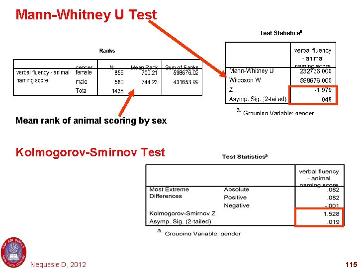
Mann-Whitney U Test Mean rank of animal scoring by sex Kolmogorov-Smirnov Test Negussie D, 2012 115