Statistical testing parametric and nonparametric tests univariate analysis
 univariate analysis, mulitple regression analysis, survival analysis; how")


. The t-test is the most commonly used method")
. Theoretically, the t-test can be used even if")
. The t-test is based on assumptions of normality")
 is to test for significant")


 and an")


, 95% Confidence Interval (CI) and P value of the association between")
 estimates comparing the subjects previously studied for chromosomal aberrations")
- Slides: 38
Statistical testing (parametric and non-parametric tests) univariate analysis, mulitple regression analysis, survival analysis; how to choose the right statistical approach) IRCCS San Raffaele Pisana, Rome, Italy, 28 February - 2 March 2018
American Statistical Association, May 2016
Univariate Analysis Univariate analysis is the simplest form of analyzing data. “Uni” means “one”, so in other words your data has only one variable. It doesn’t deal with causes or relationships (unlike regression) and it’s major purpose is to describe; it takes data, summarizes that data and finds patterns in the data. Bivariate Analysis Bivariate analysis is one of the simplest forms of quantitative (statistical) analysis. It involves the analysis of two variables (often denoted as X, Y), for the purpose of determining the empirical relationship between them. Multivariate Analysis Multivariate analysis is based on the statistical principle of multivariate statistics, which involves observation and analysis of more than one statistical outcome variable at a time. In design and analysis, the technique is used to perform trade studies across multiple dimensions while taking into account the effects of all variables on the responses of interest.
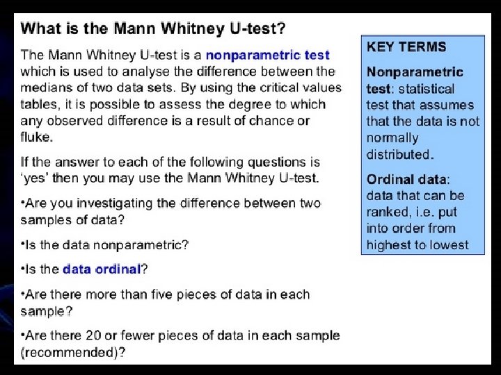
Different types of data require different statistical methods. Why? With interval data and below, operations like addition, subtraction, multiplication, and division are meaningless! Parametric statistics: - Typically take advantage of central limit theorem (imposes requirements on probability distributions) - Appropriate only for interval and ratio data. - More powerful than nonparametric methods. Nonparametric statistics: - Do not require assumptions concerning the probability distribution for the population. - There are many methods appropriate for ordinal data, some methods appropriate for nominal data. - Computations typically make use of data's ranks instead of actual data.
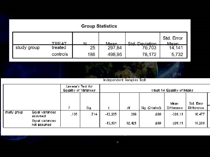
t-test (for independent and dependent samples). The t-test is the most commonly used method to evaluate the differences in means between two groups. The groups can be independent (e. g. , blood pressure of patients who were given a drug vs. a control group who received a placebo) or dependent (e. g. , blood pressure of patients "before" vs. "after" they received a drug, see below).
t-test (for independent and dependent samples). Theoretically, the t-test can be used even if the sample sizes are very small (e. g. , as small as 10; some researchers claim that even smaller sample sizes are possible), as long as the variables are approximately normally distributed and the variation of scores in the two groups is not reliably different
t-test (for independent and dependent samples). The t-test is based on assumptions of normality and homogeneity of variance. You can test for both these As long as the samples in each group are large and nearly equal, the t-test is robust, that is, still good, even the assumptions are not met.
General ANOVA. The purpose of analysis of variance (ANOVA) is to test for significant differences between means by comparing (i. e. , analyzing) variances. More specifically, by partitioning the total variation into different sources (associated with the different effects in the design), we are able to compare the variance due to the between-groups variability with that due to the within-group variability. Under the null hypothesis (that there are no mean differences between groups or treatments in the population), the variance estimated from the within-group variability should be about the same as the variance estimated from between-groups variability.
Iarmarcovai et al. , Mutat Res, 2007
Iarmarcovai et al. , Mutat Res, 2007
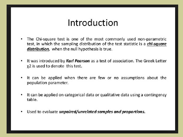
2 χ = Chi square = 3. 84 1 df P< 0. 05
Correlation is any of a broad class of statistical relationships involving dependence, though in common usage it most often refers to how close two variables are to having a linear relationship with each other Correlations are useful because they can indicate a predictive relationship that can be exploited in practice. However, in general, the presence of a correlation is not sufficient to infer the presence of a causal relationship (i. e. , correlation does not imply causation).
A correlation coefficient is a numerical measure of some type of correlation, meaning a statistical relationship between two variables. Several types of correlation coefficient exist, each with their own definition and own range of usability and characteristics. They all assume values in the range from − 1 to +1, where +1 indicates the strongest possible agreement and − 1 the strongest possible disagreement. Pearson The Pearson product-moment correlation coefficient, also known as r, R, or Pearson's r, is a measure of the strength and direction of the linear relationship between two variables. This is the best known and most commonly used type of correlation coefficient; when the term "correlation coefficient" is used without further qualification, it usually refers to the Pearson product-moment correlation coefficient
Regression analysis is a set of statistical processes for estimating the relationships among variables. It includes many techniques for modeling and analyzing several variables, when the focus is on the relationship between a dependent variable and one or more independent variables (or 'predictors'). Ŷ = α+βxn+ε
The choice of the regression model depends on the underlying statistical model and by the kind of data to be analysed. Linear data – Normally distributed Linear regression – Log-Log regression Count (i. e. , MN) Log Linear, Poisson, Negative Binomial Logistic regression Yes-No dependent variable Survival data Cox Regression
Why use logarithmic transformations of variables Logarithmically transforming variables in a regression model is a very common way to handle situations where a non-linear relationship exists between the independent and dependent variables. Using the logarithm of one or more variables instead of the un-logged form makes the effective relationship non-linear, while still preserving the linear model. A great advantage of these models (log-log linear) is the generation of mean ratio estimates Ln ŷ = α + β ln Xi + ε Assuming X = age in years Ln ŷ = α + (β ln X 10 – ln X 0) + ε ln X 10 – ln X 0 = Ln (X 10 / ln X 0 ) e Ln (X 10 / ln X 0 ) = = X 10 / X 0 = Mean Ratio (DNA Damage in 60 years) = 1. 26 (DNA Damage in 50 years)
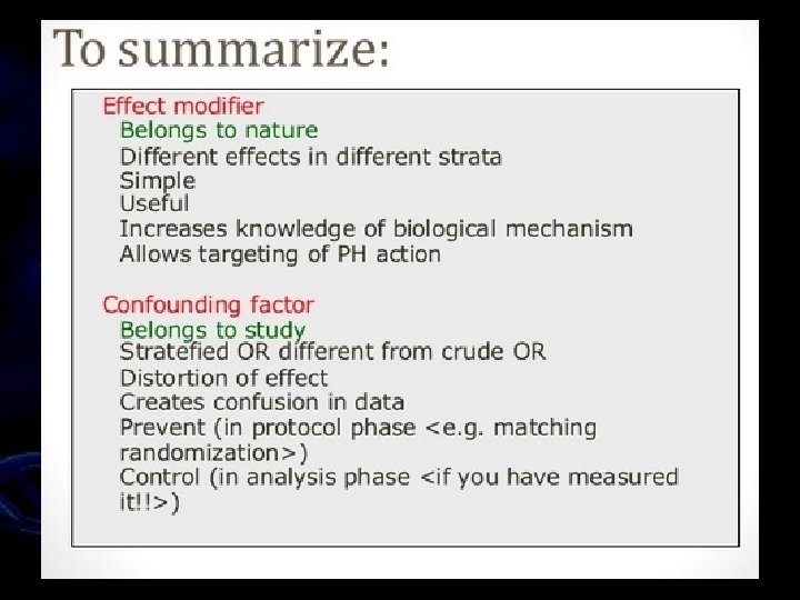
Confounding provides an alternative explanation for an association between an exposure (X) and an outcome. In order for a variable to be considered as a confounder: - The variable must be independently associated with the outcome (i. e. be a risk factor). - The variable must be also associated with the exposure under study in the source population. - It should not lie on the causal pathway between exposure and disease.
Effect modification occurs when the magnitude of the effect of the primary exposure on an outcome (i. e. , the association) differs depending on the level of a third variable. Unlike confounding, effect modification is a biological phenomenon in which the exposure has a different impact in different circumstances. It is not possible to adjust for effect modification Polymorphisms in NAT 2 related to Cancer
The common epidemiologic approach to the study of health effects recognizes as the principal aim of a study that of quantifying exposures-effect relationships, rather then simply evaluate whether an effect is present.
A point estimate of the association between exposure and effect should be computed, along with its confidence interval, so as to provide a range of values within which the true association falls with a given probability. and this concepts bring us to the measures of association !
Measures of association reflect the strength of the statistical relationship between a study factor and a disease
The most useful and widely used measures of association in Epidemiology and Clinical Investigation are: Risk difference, Incidence Rate Difference, Risk Ratio, Incidence Ratio, and Odds Ratio
Cross Sectional studies examines the relationship between a biomarker and other variables of interest as they exist in a defined population at one particular time. No matter the temporal sequence of cause and effect. Exposed Cases Exposed Controls Study Population Sample Non Exposed Cases Non Exposed Controls
Exposed Unexposed Total BMK+ a b M 1 BMK- c d M 2 Total N 1 N 2 N Let p 1 and p 2 be the proportion denoting the prevalence of the biomarkers in the exposed and unexposed groups, i. e. , Pˆ1 = a/N 1 Pˆ2 = b/N 2
Exposed Unexposed Total BMK+ a b M 1 BMK- c d M 2 Total N 1 N 2 N Prevalence Difference: PD = P 1 - P 2 Prevalence Ratio: PR = P 1 /P 2 P 1 = a/N 1 P 2 = b/N 2
Exposed Unexposed Total BMK+ a b M 1 BMK- c d M 2 Total N 1 N 2 N Odds Ratio = P 1 /(1 - P 1) P 2 /(1 - P 2) = (a/N 1)/(c/N 1) (b/N 2)/(d/N 2) = ad bc
Cross Sectional study Parameters and sample properties are identical with those from prospective studies RD = P 1 - P 2 RR = P 1 /P 2 POR = P 1 /(1 - P 1) P 2 /(1 - P 2) Instead of Mesures of Risk we have Mesures of Prevalence Exposed Unexposed Total BMK+ a b M 1 BMK- c d M 2 Total N 1 N 2 N
Cross Sectional study It’s a measure of association – Based on the logit model RD = P 1 - P 2 RR = P 1 /P 2 POR = P 1 /(1 - P 1) P 2 /(1 - P 2) Exposed Unexposed It expresses a causeeffect relationship Not evaluable in a cross-sectional design Total BMK+ a b M 1 BMK- c d M 2 Total N 1 N 2 N
Cross Sectional study RD = P 1 - P 2 RR = P 1 /P 2 POR = P 1 /(1 - P 1) P 2 /(1 - P 2) (RR = (a/M 1)/(b/M 2)) EOR = P 1 /(1 - P 1) P 2 /(1 - P 2) Case-Control study Exposed Unexposed Total BMK+ a b M 1 BMK- c d M 2 Total N 1 N 2 N
Cross Sectional study Cohort study RD = P 1 - P 2 RR = P 1 /P 2 POR = P 1 /(1 - P 1) P 2 /(1 - P 2) (RR = (a/M 1)/(b/M 2)) EOR = P 1 /(1 - P 1) P 2 /(1 - P 2) Case-Control study RD = P 1 - P 2 IDR = RR = CIR = RR = P 1 /P 2 ROR = P 1 /(1 - P 1) P 2 /(1 - P 2) Exposed Unexposed Total BMK+ a b M 1 BMK- c d M 2 Total N 1 N 2 N
Hadjidekova et. al, 2001
Odd Ratios (OR), 95% Confidence Interval (CI) and P value of the association between genetic polymorphisms and Malignant Pleural Mesothelioma Gender Cases Controls n. (%) Men 74 (82. 2) 217 (54. 9) Women 16 (17. 8) 178 (45. 1) Cases Contr. OR* 95% CI P GSTT 1 Functional Null 71 17 317 70 1 1. 31 0. 71 -2. 43 0. 391 Mn. SOD V 16 A Homozygotes Val/Val Heterozygotes Ala/Val Homozygotes Ala/Ala 16 27 37 98 170 81 1 0. 99 3. 07 0. 50 -1. 96 1. 55 -6. 05 0. 968 0. 001 * ORs adjusted by gender and age (Logistic regression) Polymorphisms of glutathione-S-transferase M 1 and superoxide dismutase affect the risk of malignant pleural mesothelioma. Landi et al. , int J cancer
Total cancer incidence ratio (IR) estimates comparing the subjects previously studied for chromosomal aberrations (CAs), chromatid-type aberrations (CTAs), and chromosome-type aberrations (CSAs) Hagmar et. al, 2004