Parametric Nonparametric Univariate Statistics Univariate Significance Tests Tests

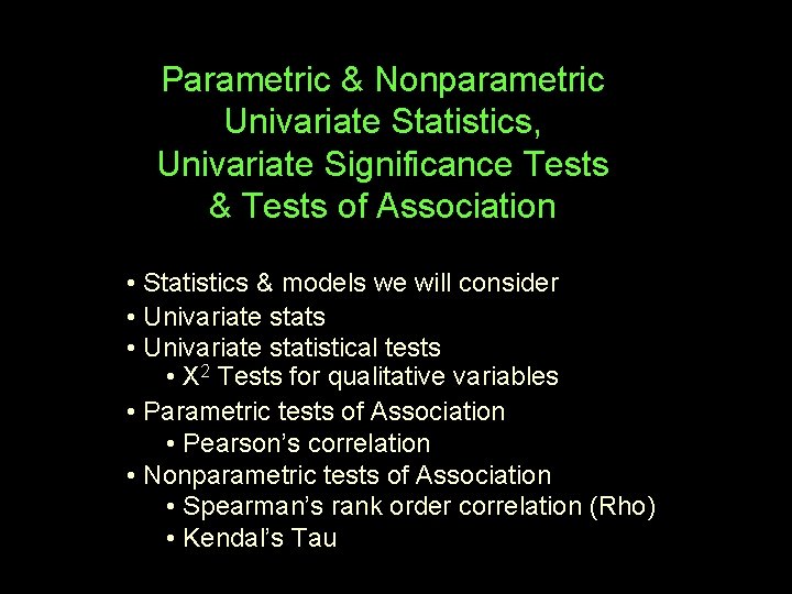
Parametric & Nonparametric Univariate Statistics, Univariate Significance Tests & Tests of Association • Statistics & models we will consider • Univariate stats • Univariate statistical tests • X 2 Tests for qualitative variables • Parametric tests of Association • Pearson’s correlation • Nonparametric tests of Association • Spearman’s rank order correlation (Rho) • Kendal’s Tau

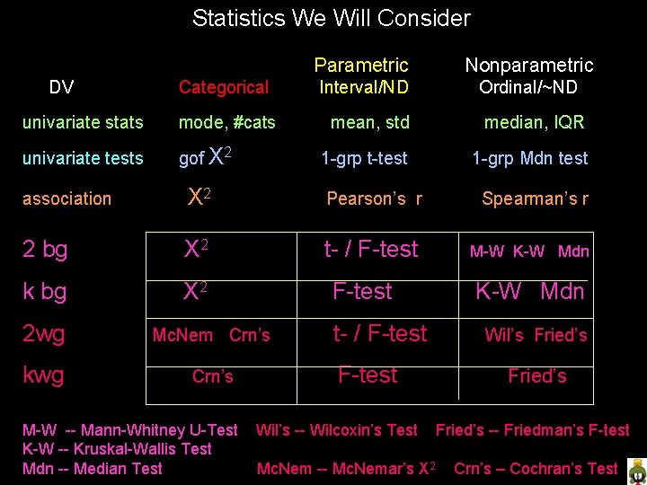
Statistics We Will Consider DV Categorical univariate stats mode, #cats univariate tests gof X 2 Parametric Nonparametric Interval/ND Ordinal/~ND mean, std median, IQR 1 -grp t-test 1 -grp Mdn test association X 2 Pearson’s r Spearman’s r 2 bg X 2 t- / F-test M-W K-W Mdn k bg X 2 F-test 2 wg Mc. Nem Crn’s kwg Crn’s M-W -- Mann-Whitney U-Test K-W -- Kruskal-Wallis Test Mdn -- Median Test t- / F-test Wil’s -- Wilcoxin’s Test Mc. Nem -- Mc. Nemar’s X 2 K-W Mdn Wil’s Fried’s -- Friedman’s F-test Crn’s – Cochran’s Test

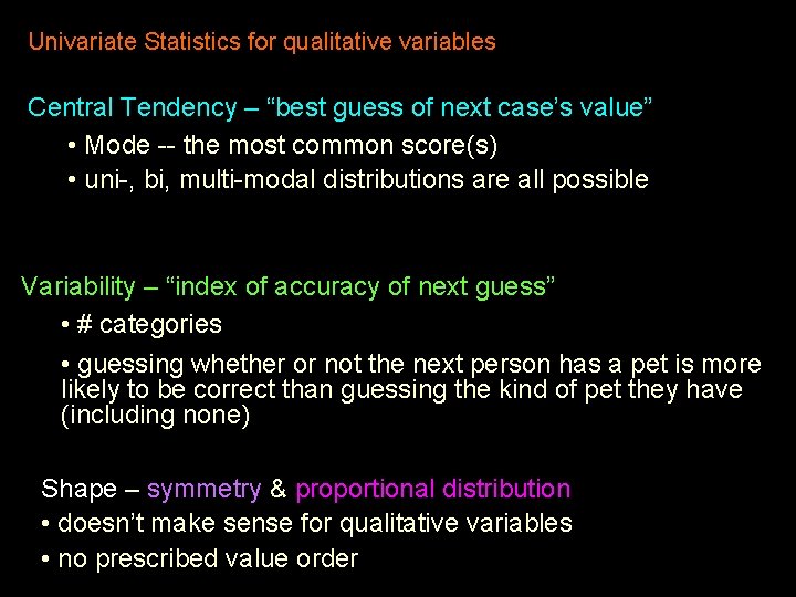
Univariate Statistics for qualitative variables Central Tendency – “best guess of next case’s value” • Mode -- the most common score(s) • uni-, bi, multi-modal distributions are all possible Variability – “index of accuracy of next guess” • # categories • guessing whether or not the next person has a pet is more likely to be correct than guessing the kind of pet they have (including none) Shape – symmetry & proportional distribution • doesn’t make sense for qualitative variables • no prescribed value order

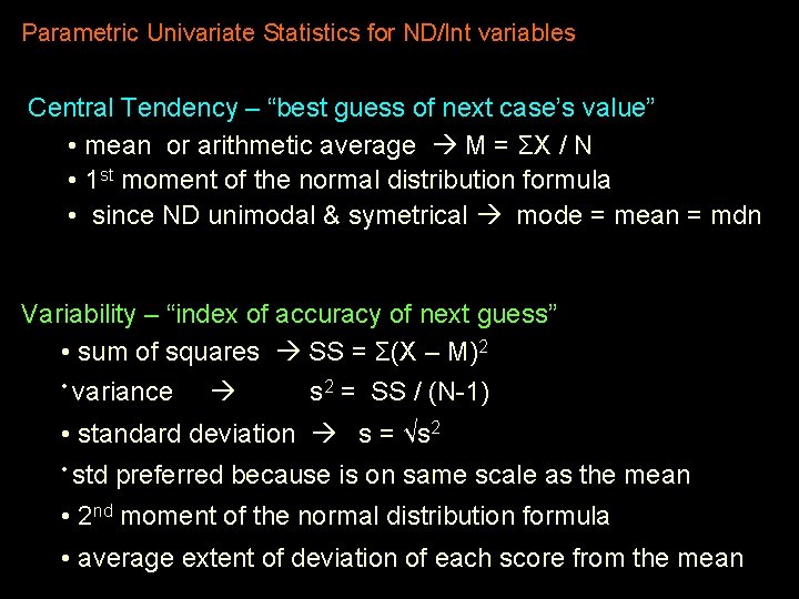
Parametric Univariate Statistics for ND/Int variables Central Tendency – “best guess of next case’s value” • mean or arithmetic average M = ΣX / N • 1 st moment of the normal distribution formula • since ND unimodal & symetrical mode = mean = mdn Variability – “index of accuracy of next guess” • sum of squares SS = Σ(X – M)2 • variance s 2 = SS / (N-1) • standard deviation s = √s 2 • std preferred because is on same scale as the mean • 2 nd moment of the normal distribution formula • average extent of deviation of each score from the mean

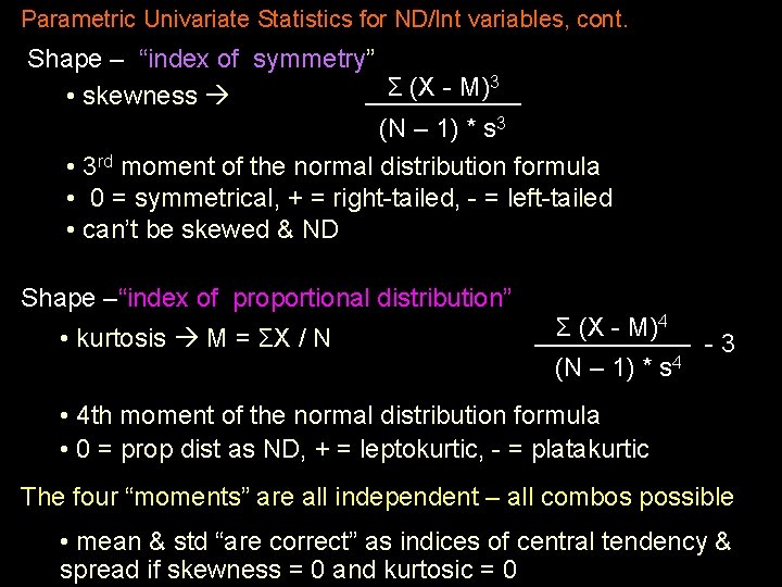
Parametric Univariate Statistics for ND/Int variables, cont. Shape – “index of symmetry” 3 Σ (X M) • skewness (N – 1) * s 3 • 3 rd moment of the normal distribution formula • 0 = symmetrical, + = right-tailed, - = left-tailed • can’t be skewed & ND Shape –“index of proportional distribution” • kurtosis M = ΣX / N Σ (X - M)4 (N – 1) * s 4 -3 • 4 th moment of the normal distribution formula • 0 = prop dist as ND, + = leptokurtic, - = platakurtic The four “moments” are all independent – all combos possible • mean & std “are correct” as indices of central tendency & spread if skewness = 0 and kurtosic = 0

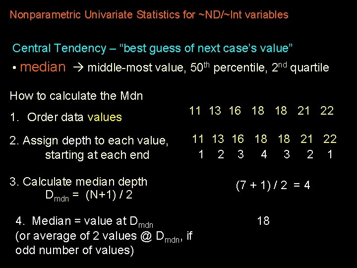
Nonparametric Univariate Statistics for ~ND/~Int variables Central Tendency – “best guess of next case’s value” • median middle-most value, 50 th percentile, 2 nd quartile How to calculate the Mdn 1. Order data values 2. Assign depth to each value, starting at each end 11 13 16 18 18 21 22 1 2 3 4 3 2 1 3. Calculate median depth Dmdn = (N+1) / 2 4. Median = value at Dmdn (or average of 2 values @ Dmdn, if odd number of values) (7 + 1) / 2 = 4 18

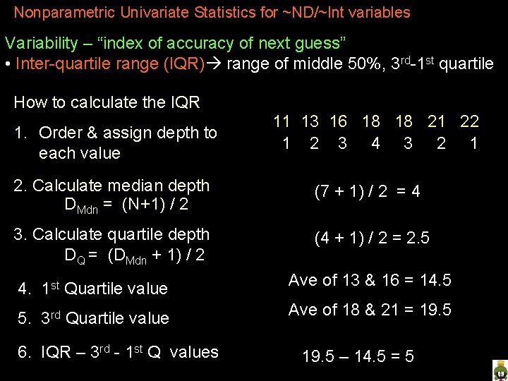
Nonparametric Univariate Statistics for ~ND/~Int variables Variability – “index of accuracy of next guess” • Inter-quartile range (IQR) range of middle 50%, 3 rd-1 st quartile How to calculate the IQR 1. Order & assign depth to each value 11 13 16 18 18 21 22 1 2 3 4 3 2 1 2. Calculate median depth DMdn = (N+1) / 2 (7 + 1) / 2 = 4 3. Calculate quartile depth DQ = (DMdn + 1) / 2 (4 + 1) / 2 = 2. 5 4. 1 st Quartile value Ave of 13 & 16 = 14. 5 5. 3 rd Quartile value Ave of 18 & 21 = 19. 5 6. IQR – 3 rd - 1 st Q values 19. 5 – 14. 5 = 5

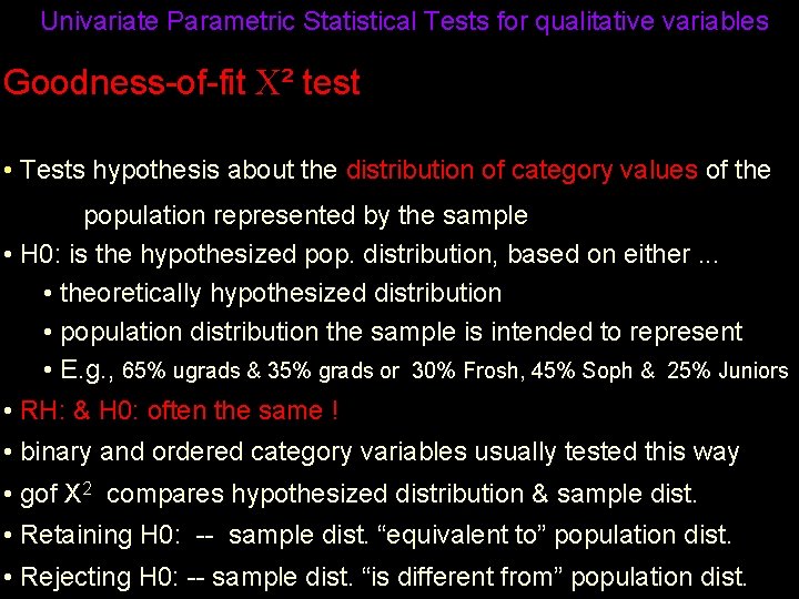
Univariate Parametric Statistical Tests for qualitative variables Goodness-of-fit ² test • Tests hypothesis about the distribution of category values of the population represented by the sample • H 0: is the hypothesized pop. distribution, based on either. . . • theoretically hypothesized distribution • population distribution the sample is intended to represent • E. g. , 65% ugrads & 35% grads or 30% Frosh, 45% Soph & 25% Juniors • RH: & H 0: often the same ! • binary and ordered category variables usually tested this way • gof X 2 compares hypothesized distribution & sample dist. • Retaining H 0: -- sample dist. “equivalent to” population dist. • Rejecting H 0: -- sample dist. “is different from” population dist.

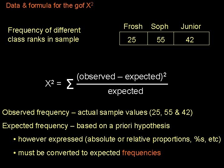
Data & formula for the gof X 2 Frequency of different class ranks in sample X 2 = Σ Frosh Soph Junior 25 55 42 (observed – expected)2 expected Observed frequency – actual sample values (25, 55 & 42) Expected frequency – based on a priori hypothesis • however expressed (absolute or relative proportions, %s, etc) • must be converted to expected frequencies

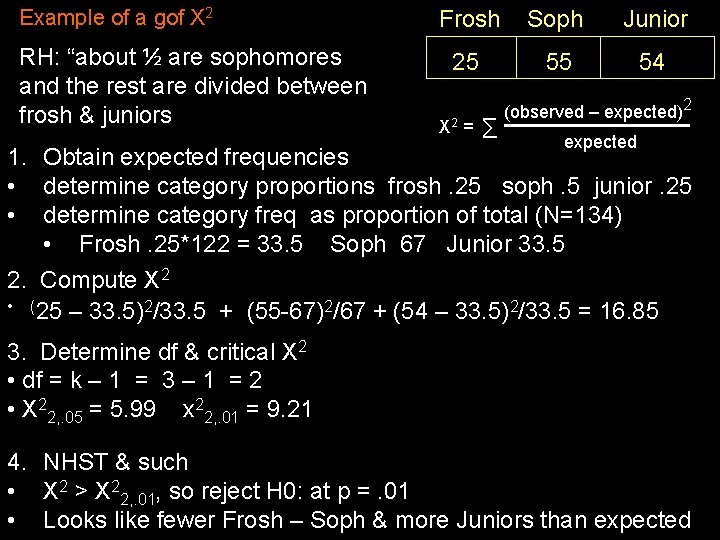
Example of a gof X 2 RH: “about ½ are sophomores and the rest are divided between frosh & juniors Frosh Soph Junior 25 55 54 X 2 = Σ (observed – expected)2 expected 1. Obtain expected frequencies • determine category proportions frosh. 25 soph. 5 junior. 25 • determine category freq as proportion of total (N=134) • Frosh. 25*122 = 33. 5 Soph 67 Junior 33. 5 2. Compute X 2 • (25 – 33. 5)2/33. 5 + (55 -67)2/67 + (54 – 33. 5)2/33. 5 = 16. 85 3. Determine df & critical X 2 • df = k – 1 = 3 – 1 = 2 • X 22, . 05 = 5. 99 x 22, . 01 = 9. 21 4. NHST & such • X 2 > X 22, . 01, so reject H 0: at p =. 01 • Looks like fewer Frosh – Soph & more Juniors than expected

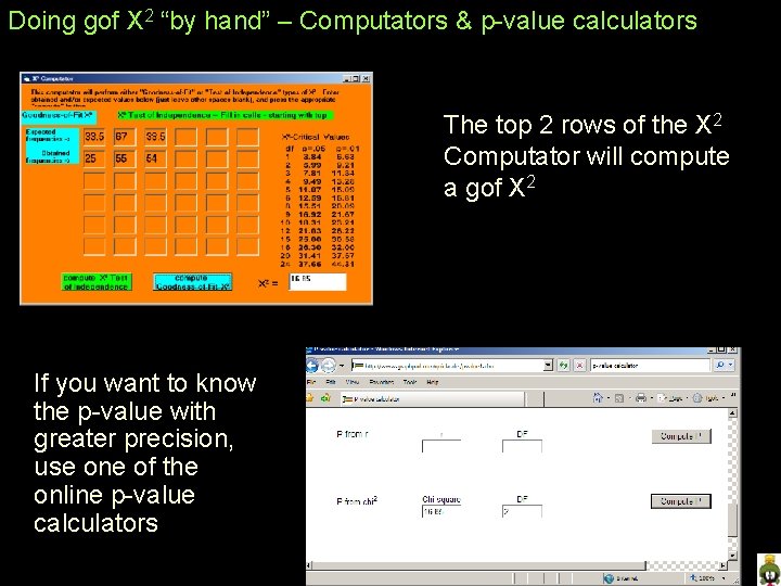
Doing gof X 2 “by hand” – Computators & p-value calculators The top 2 rows of the X 2 Computator will compute a gof X 2 If you want to know the p-value with greater precision, use one of the online p-value calculators

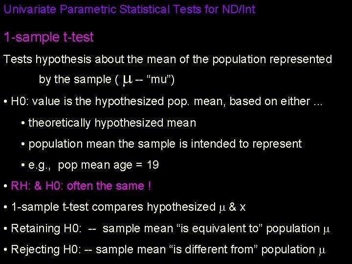
Univariate Parametric Statistical Tests for ND/Int 1 -sample t-test Tests hypothesis about the mean of the population represented by the sample ( -- “mu”) • H 0: value is the hypothesized pop. mean, based on either. . . • theoretically hypothesized mean • population mean the sample is intended to represent • e. g. , pop mean age = 19 • RH: & H 0: often the same ! • 1 -sample t-test compares hypothesized & x • Retaining H 0: -- sample mean “is equivalent to” population • Rejecting H 0: -- sample mean “is different from” population

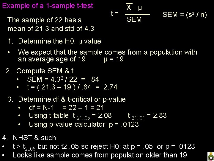
Example of a 1 -sample t-test The sample of 22 has a mean of 21. 3 and std of 4. 3 t= X-µ SEM = (s² / n) 1. Determine the H 0: µ value • We expect that the sample comes from a population with an average of 19 µ = 19 2. Compute SEM & t • SEM = 4. 32 / 22 =. 84 • t = ( 21. 3 – 19 ) /. 84 = 2. 74 3. Determine df & t-critical or p-value • df = N-1 = 22 – 1 = 21 • Using t-table t 21, . 05 = 2. 08 t 21, . 01 = 2. 83 • Using p-value calculator p =. 0123 4. NHST & such • t > t 2, . 05 but not t 2, . 05 so reject H 0: at p =. 05 or p =. 0123 • Looks like sample comes from population older than 19

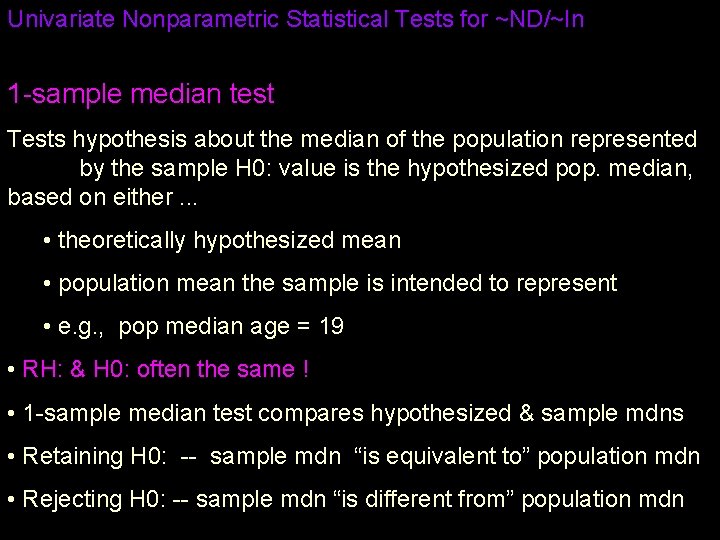
Univariate Nonparametric Statistical Tests for ~ND/~In 1 -sample median test Tests hypothesis about the median of the population represented by the sample H 0: value is the hypothesized pop. median, based on either. . . • theoretically hypothesized mean • population mean the sample is intended to represent • e. g. , pop median age = 19 • RH: & H 0: often the same ! • 1 -sample median test compares hypothesized & sample mdns • Retaining H 0: -- sample mdn “is equivalent to” population mdn • Rejecting H 0: -- sample mdn “is different from” population mdn

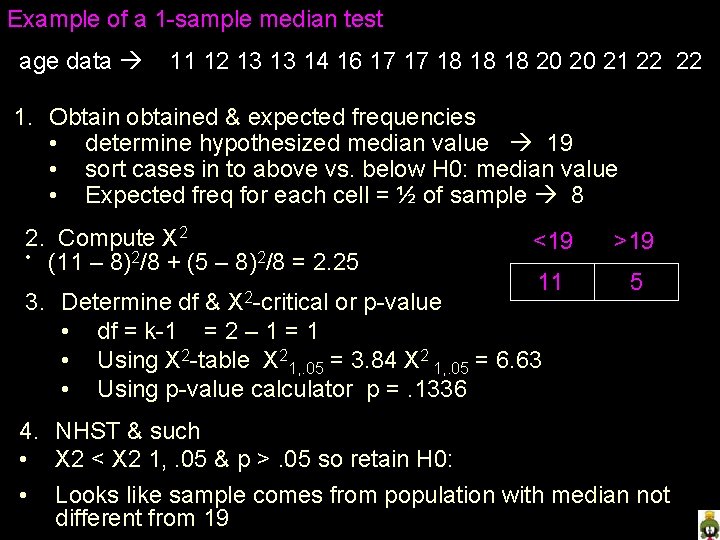
Example of a 1 -sample median test age data 11 12 13 13 14 16 17 17 18 18 18 20 20 21 22 22 1. Obtain obtained & expected frequencies • determine hypothesized median value 19 • sort cases in to above vs. below H 0: median value • Expected freq for each cell = ½ of sample 8 2. Compute X 2 • (11 – 8)2/8 + (5 – 8)2/8 = 2. 25 <19 >19 11 5 3. Determine df & or p-value • df = k-1 = 2 – 1 = 1 • Using X 2 -table X 21, . 05 = 3. 84 X 2 1, . 05 = 6. 63 • Using p-value calculator p =. 1336 X 2 -critical 4. NHST & such • X 2 < X 2 1, . 05 & p >. 05 so retain H 0: • Looks like sample comes from population with median not different from 19

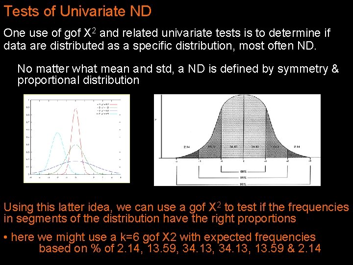
Tests of Univariate ND One use of gof X 2 and related univariate tests is to determine if data are distributed as a specific distribution, most often ND. No matter what mean and std, a ND is defined by symmetry & proportional distribution Using this latter idea, we can use a gof X 2 to test if the frequencies in segments of the distribution have the right proportions • here we might use a k=6 gof X 2 with expected frequencies based on % of 2. 14, 13. 59, 34. 13, 13. 59 & 2. 14

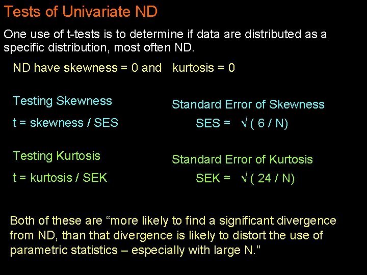
Tests of Univariate ND One use of t-tests is to determine if data are distributed as a specific distribution, most often ND. ND have skewness = 0 and kurtosis = 0 Testing Skewness t = skewness / SES Standard Error of Skewness SES ≈ √ ( 6 / N) Testing Kurtosis Standard Error of Kurtosis t = kurtosis / SEK ≈ √ ( 24 / N) Both of these are “more likely to find a significant divergence from ND, than that divergence is likely to distort the use of parametric statistics – especially with large N. ”

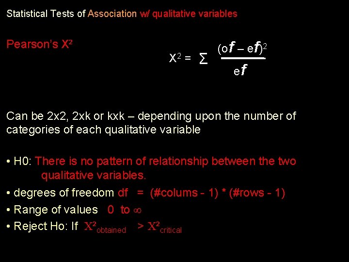
Statistical Tests of Association w/ qualitative variables Pearson’s X² X 2 = Σ (of – ef)2 ef Can be 2 x 2, 2 xk or kxk – depending upon the number of categories of each qualitative variable • H 0: There is no pattern of relationship between the two qualitative variables. • degrees of freedom df = (#colums - 1) * (#rows - 1) • Range of values 0 to • Reject Ho: If ²obtained > ²critical

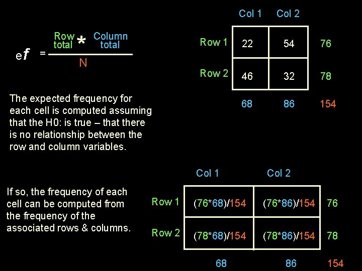
Col 1 ef = Row total *N Column total Row 1 22 54 76 Row 2 46 32 78 68 86 154 The expected frequency for each cell is computed assuming that the H 0: is true – that there is no relationship between the row and column variables. Col 1 If so, the frequency of each cell can be computed from the frequency of the associated rows & columns. Col 2 Row 1 (76*68)/154 (76*86)/154 76 Row 2 (78*68)/154 (78*86)/154 78 68 86 154

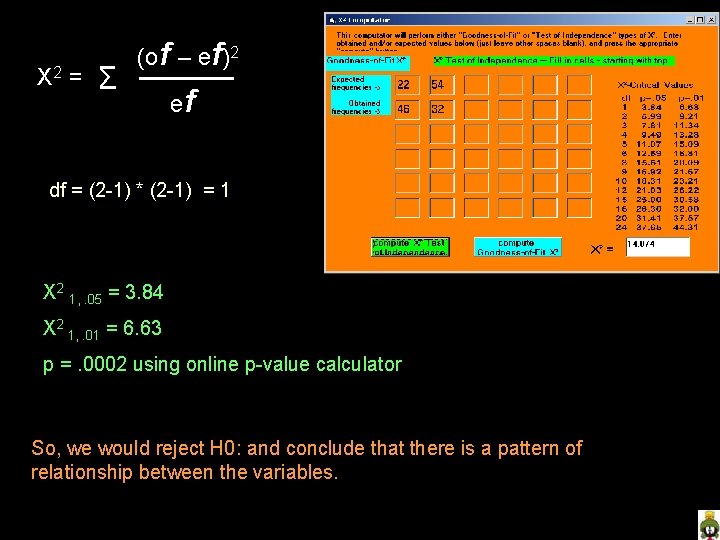
X 2 = Σ (of – ef)2 ef df = (2 -1) * (2 -1) = 1 X 2 1, . 05 = 3. 84 X 2 1, . 01 = 6. 63 p =. 0002 using online p-value calculator So, we would reject H 0: and conclude that there is a pattern of relationship between the variables.

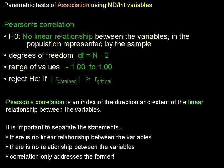
Parametric tests of Association using ND/Int variables Pearson’s correlation • H 0: No linear relationship between the variables, in the population represented by the sample. • degrees of freedom df = N - 2 • range of values - 1. 00 to 1. 00 • reject Ho: If | robtained | > rcritical Pearson’s correlation is an index of the direction and extent of the linear relationship between the variables. It is important to separate the statements… • there is no linear relationship between the variables • there is no relationship between the variables • correlation only addresses the former!

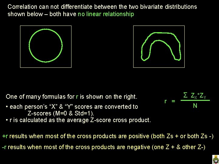
Correlation can not differentiate between the two bivariate distributions shown below – both have no linear relationship One of many formulas for r is shown on the right. • each person’s “X” & “Y” scores are converted to Z-scores (M=0 & Std=1). • r is calculated as the average Z-score cross product. r = Σ ZX*ZY N +r results when most of the cross products are positive (both Zs + or both Zs -) -r results when most of the cross products are negative (one Z + & other Z-)

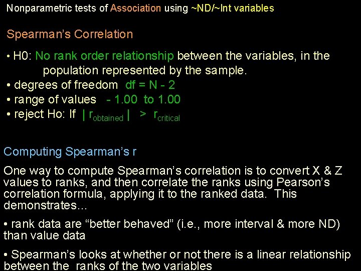
Nonparametric tests of Association using ~ND/~Int variables Spearman’s Correlation • H 0: No rank order relationship between the variables, in the population represented by the sample. • degrees of freedom df = N - 2 • range of values - 1. 00 to 1. 00 • reject Ho: If | robtained | > rcritical Computing Spearman’s r One way to compute Spearman’s correlation is to convert X & Z values to ranks, and then correlate the ranks using Pearson’s correlation formula, applying it to the ranked data. This demonstrates… • rank data are “better behaved” (i. e. , more interval & more ND) than value data • Spearman’s looks at whether or not there is a linear relationship between the ranks of the two variables

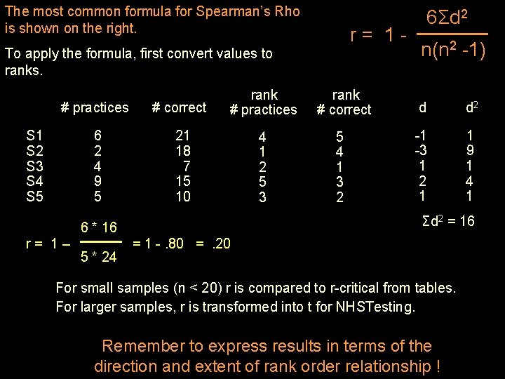
The most common formula for Spearman’s Rho is shown on the right. r= 1 - To apply the formula, first convert values to ranks. # practices # correct rank # practices 6 2 4 9 5 21 18 7 15 10 4 1 2 5 3 S 1 S 2 S 3 S 4 S 5 5 * 24 n(n 2 -1) rank # correct d d 2 5 4 1 3 2 -1 -3 1 2 1 1 9 1 4 1 Σd 2 = 16 6 * 16 r= 1– 6Σd 2 = 1 -. 80 =. 20 For small samples (n < 20) r is compared to r-critical from tables. For larger samples, r is transformed into t for NHSTesting. Remember to express results in terms of the direction and extent of rank order relationship !

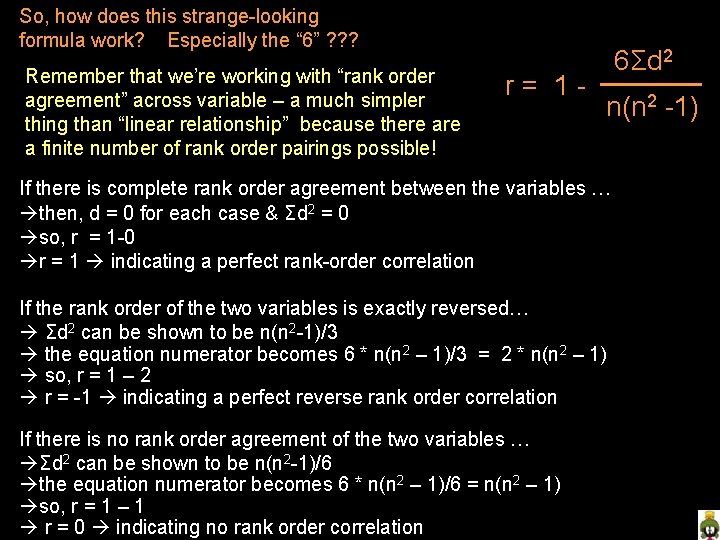
So, how does this strange-looking formula work? Especially the “ 6” ? ? ? Remember that we’re working with “rank order agreement” across variable – a much simpler thing than “linear relationship” because there a finite number of rank order pairings possible! r= 1 - 6Σd 2 n(n 2 -1) If there is complete rank order agreement between the variables … then, d = 0 for each case & Σd 2 = 0 so, r = 1 -0 r = 1 indicating a perfect rank-order correlation If the rank order of the two variables is exactly reversed… Σd 2 can be shown to be n(n 2 -1)/3 the equation numerator becomes 6 * n(n 2 – 1)/3 = 2 * n(n 2 – 1) so, r = 1 – 2 r = -1 indicating a perfect reverse rank order correlation If there is no rank order agreement of the two variables … Σd 2 can be shown to be n(n 2 -1)/6 the equation numerator becomes 6 * n(n 2 – 1)/6 = n(n 2 – 1) so, r = 1 – 1 r = 0 indicating no rank order correlation

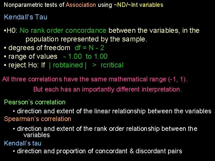
Nonparametric tests of Association using ~ND/~Int variables Kendall’s Tau • H 0: No rank order concordance between the variables, in the population represented by the sample. • degrees of freedom df = N - 2 • range of values - 1. 00 to 1. 00 • reject Ho: If | robtained | > rcritical All three correlations have the same mathematical range (-1, 1). But each has an importantly different interpretation. Pearson’s correlation • direction and extent of the linear relationship between the variables Spearman’s correlation • direction and extent of the rank order relationship between the variables Kendall’s tau • direction and proportion of concordant & discordant pairs

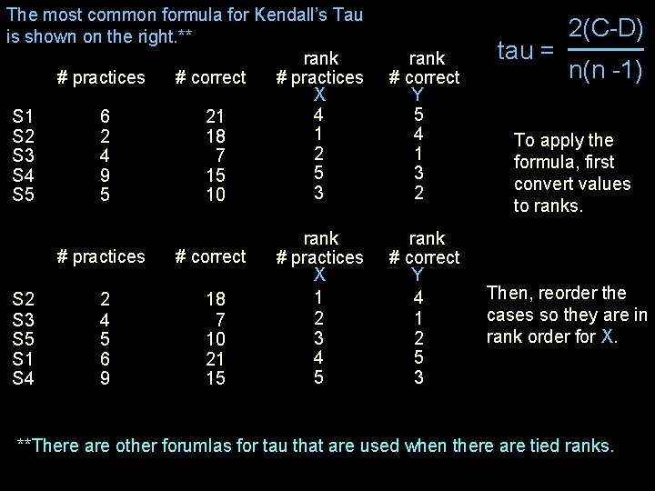
The most common formula for Kendall’s Tau is shown on the right. ** rank # practices # correct # practices X 4 S 1 6 21 1 S 2 2 18 2 S 3 4 7 5 S 4 9 15 3 S 5 5 10 rank # correct Y 5 4 1 3 2 rank # practices X 1 2 3 4 5 rank # correct Y 4 1 2 5 3 S 2 S 3 S 5 S 1 S 4 # practices # correct 2 4 5 6 9 18 7 10 21 15 tau = 2(C-D) n(n -1) To apply the formula, first convert values to ranks. Then, reorder the cases so they are in rank order for X. **There are other forumlas for tau that are used when there are tied ranks.

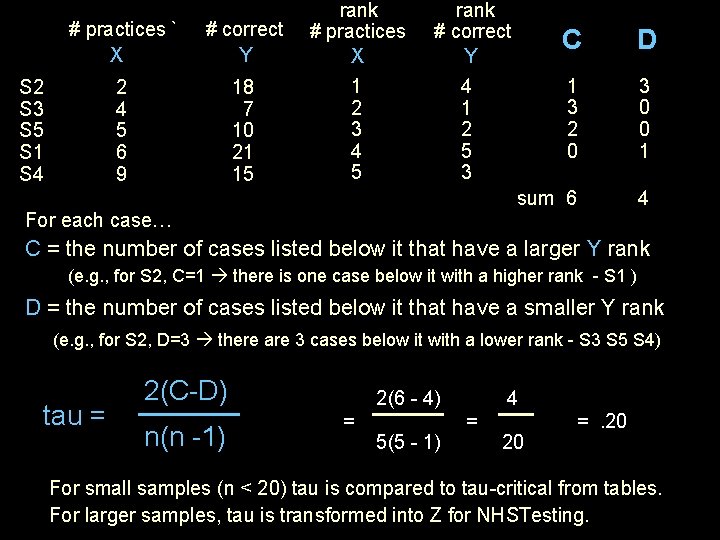
# practices ` X # correct Y rank # practices X 2 4 5 6 9 18 7 10 21 15 1 2 3 4 5 S 2 S 3 S 5 S 1 S 4 rank # correct Y 4 1 2 5 3 For each case… C D 1 3 2 0 3 0 0 1 sum 6 4 C = the number of cases listed below it that have a larger Y rank (e. g. , for S 2, C=1 there is one case below it with a higher rank - S 1 ) D = the number of cases listed below it that have a smaller Y rank (e. g. , for S 2, D=3 there are 3 cases below it with a lower rank - S 3 S 5 S 4) tau = 2(C-D) n(n -1) 2(6 - 4) = 5(5 - 1) 4 = 20 =. 20 For small samples (n < 20) tau is compared to tau-critical from tables. For larger samples, tau is transformed into Z for NHSTesting.