Multiple Regression Analysis WrapUp More Extensions of MRA

Multiple Regression Analysis: Wrap-Up More Extensions of MRA 1

Contents for Today n Probing interactions in MRA: q q q n n n Reliability and interactions Enter Method vs. Hierarchical Patterns of interactions/effects coefficients Polynomial Regression Interpretation issues in MRA Model Comparisons 2

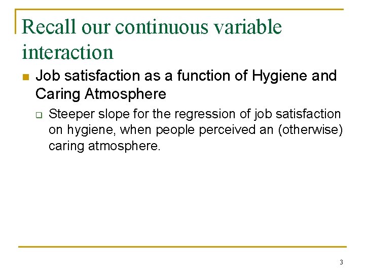
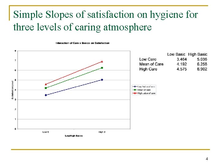
Recall our continuous variable interaction n Job satisfaction as a function of Hygiene and Caring Atmosphere q Steeper slope for the regression of job satisfaction on hygiene, when people perceived an (otherwise) caring atmosphere. 3

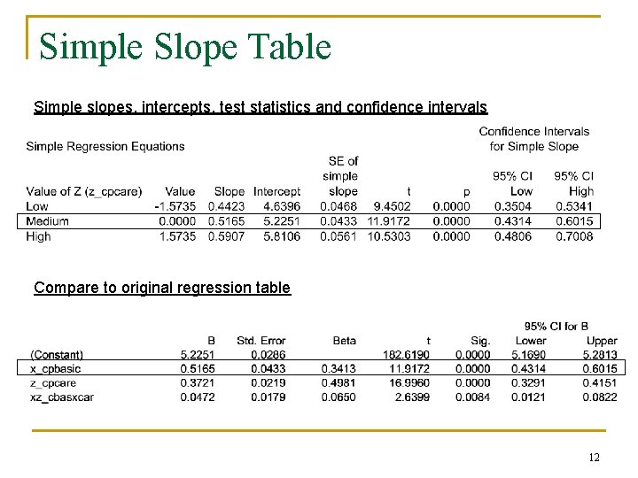
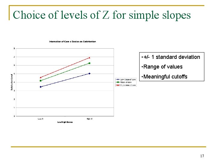
Simple Slopes of satisfaction on hygiene for three levels of caring atmosphere 4

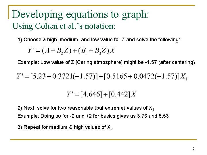
Developing equations to graph: Using Cohen et al. ’s notation: 1) Choose a high, medium, and low value for Z and solve the following: Example: Low value of Z [Caring atmosphere] might be -1. 57 (after centering) 2) Next, solve for two reasonable (but extreme) values of X 1 Example: Doing so for -2 and +2 for basics gives us 3. 76 and 5. 53 3) Repeat for medium & high values of X 2 5

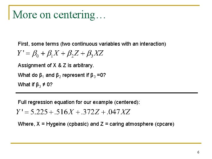
More on centering… First, some terms (two continuous variables with an interaction) Assignment of X & Z is arbitrary. What do β 1 and β 2 represent if β 3 =0? What if β 3 ≠ 0? Full regression equation for our example (centered): Where, X = Hygeine (cpbasic) and Z = caring atmosphere (cpcare) 6

Even more on centering n n n We know that centering helps us with multicollinearity issues. Let’s examine some other properties, first turning to p. 259 of reading… Note the regression equation above graph A. q Then above graph B. 7

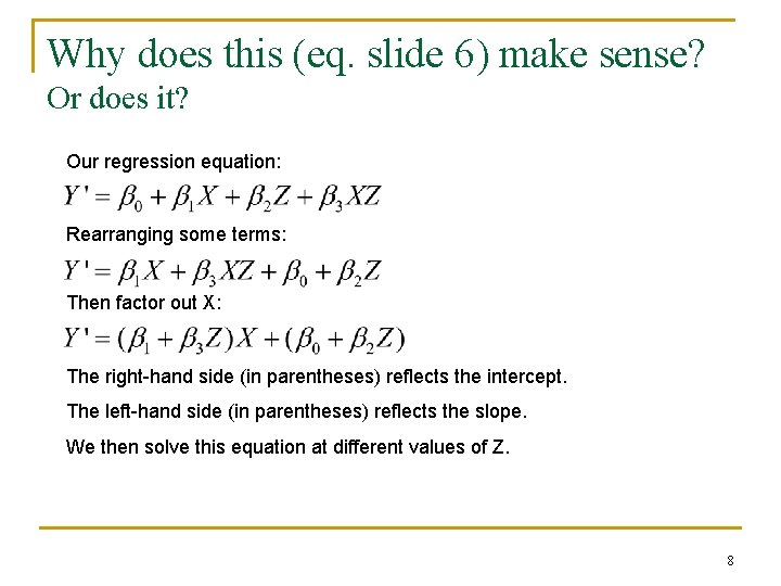
Why does this (eq. slide 6) make sense? Or does it? Our regression equation: Rearranging some terms: Then factor out X: The right-hand side (in parentheses) reflects the intercept. The left-hand side (in parentheses) reflects the slope. We then solve this equation at different values of Z. 8

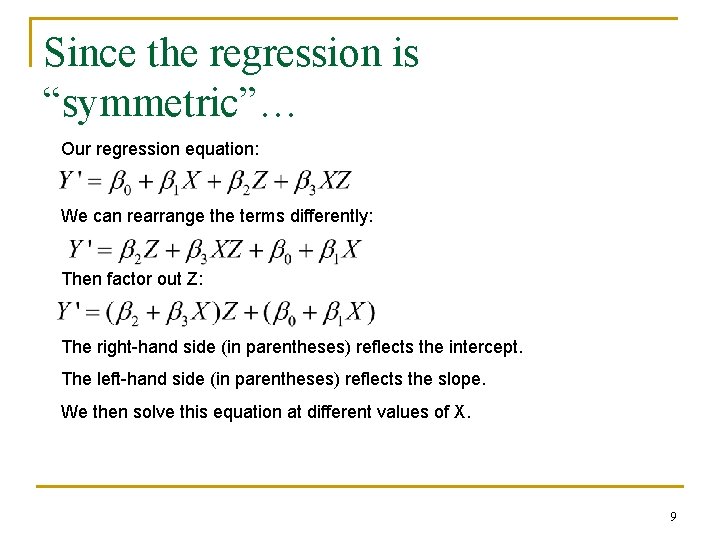
Since the regression is “symmetric”… Our regression equation: We can rearrange the terms differently: Then factor out Z: The right-hand side (in parentheses) reflects the intercept. The left-hand side (in parentheses) reflects the slope. We then solve this equation at different values of X. 9

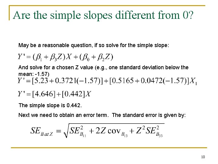
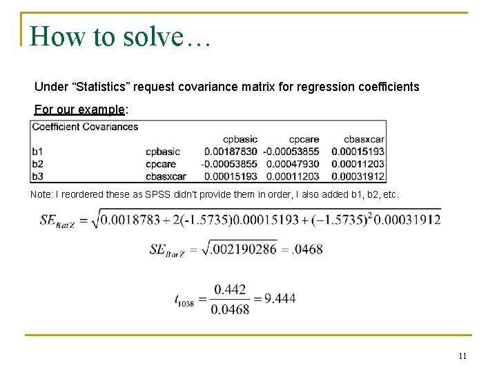
Are the simple slopes different from 0? May be a reasonable question, if so solve for the simple slope: And solve for a chosen Z value (e. g. , one standard deviation below the mean: -1. 57) The simple slope is 0. 442. Next we need to obtain an error term. The standard error is given by: 10

How to solve… Under “Statistics” request covariance matrix for regression coefficients For our example: Note: I reordered these as SPSS didn’t provide them in order, I also added b 1, b 2, etc. 11

Simple Slope Table Simple slopes, intercepts, test statistics and confidence intervals Compare to original regression table 12

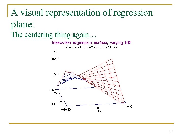
A visual representation of regression plane: The centering thing again… 13

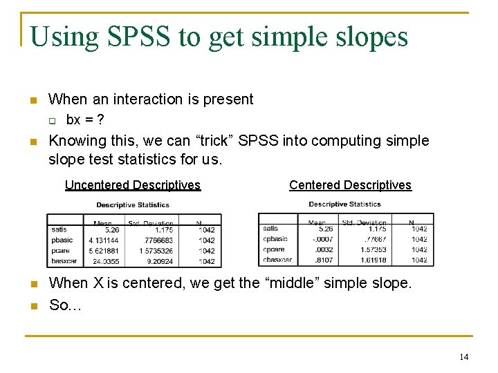
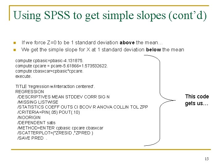
Using SPSS to get simple slopes n When an interaction is present q n bx = ? Knowing this, we can “trick” SPSS into computing simple slope test statistics for us. Uncentered Descriptives n n Centered Descriptives When X is centered, we get the “middle” simple slope. So… 14

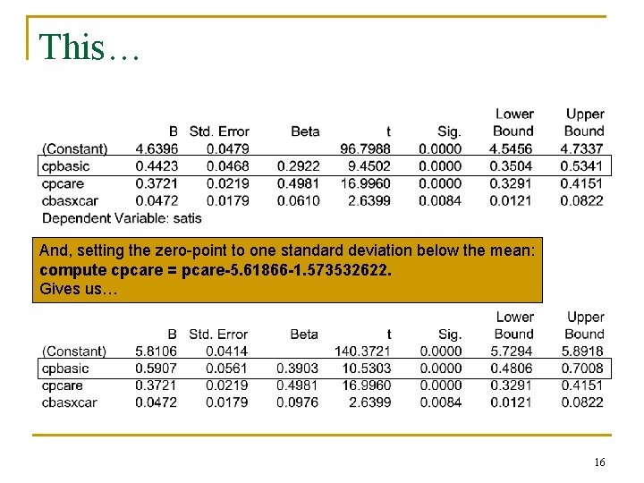
Using SPSS to get simple slopes (cont’d) n n If we force Z=0 to be 1 standard deviation above the mean… We get the simple slope for X at 1 standard deviation below the mean compute cpbasic=pbasic-4. 131875. compute cpcare = pcare-5. 61866+1. 573532622. compute cbasxcar=cpbasic*cpcare. execute. TITLE 'regression w/interaction centered'. REGRESSION /DESCRIPTIVES MEAN STDDEV CORR SIG N /MISSING LISTWISE /STATISTICS COEFF OUTS CI BCOV R ANOVA COLLIN TOL ZPP /CRITERIA=PIN(. 05) POUT(. 10) /NOORIGIN /DEPENDENT satis /METHOD=ENTER cpbasic cpcare cbasxcar /SCATTERPLOT=(*ZRESID , *ZPRED ) /SAVE PRED. This code gets us… 15

This… And, setting the zero-point to one standard deviation below the mean: compute cpcare = pcare-5. 61866 -1. 573532622. Gives us… 16

Choice of levels of Z for simple slopes • +/- 1 standard deviation • Range of values • Meaningful cutoffs 17

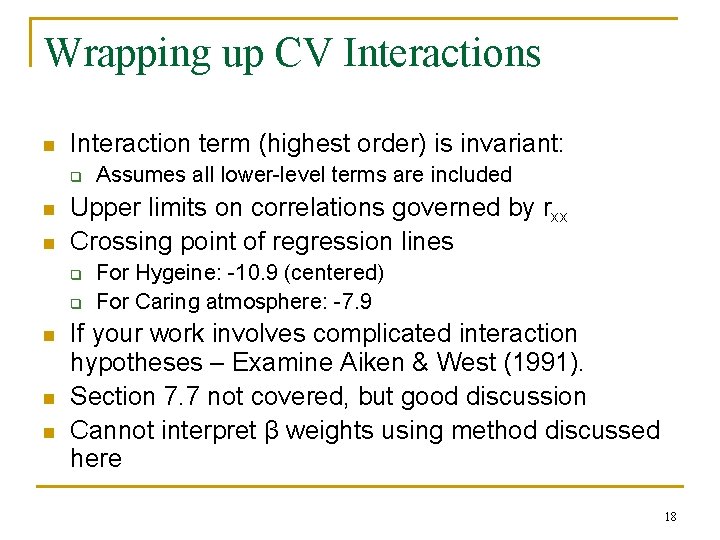
Wrapping up CV Interactions n Interaction term (highest order) is invariant: q n n Upper limits on correlations governed by rxx Crossing point of regression lines q q n n n Assumes all lower-level terms are included For Hygeine: -10. 9 (centered) For Caring atmosphere: -7. 9 If your work involves complicated interaction hypotheses – Examine Aiken & West (1991). Section 7. 7 not covered, but good discussion Cannot interpret β weights using method discussed here 18

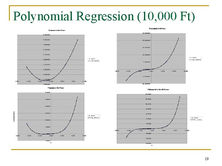
Polynomial Regression (10, 000 Ft) 19

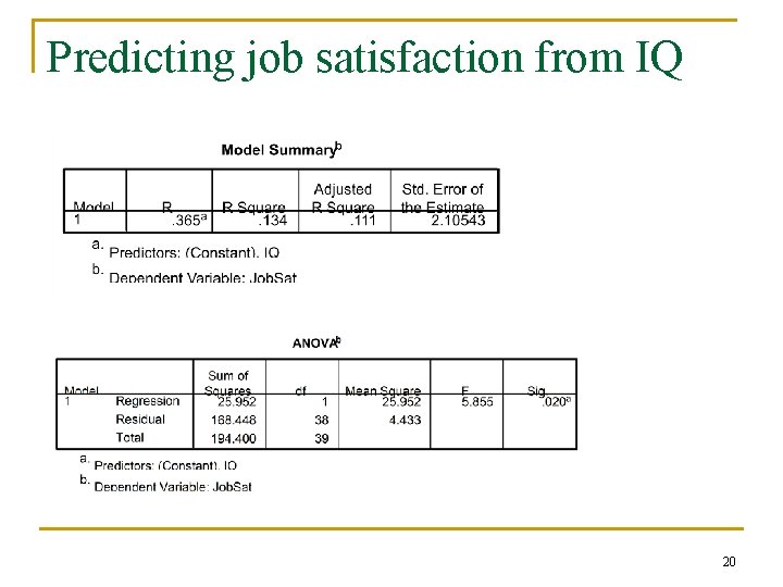
Predicting job satisfaction from IQ 20

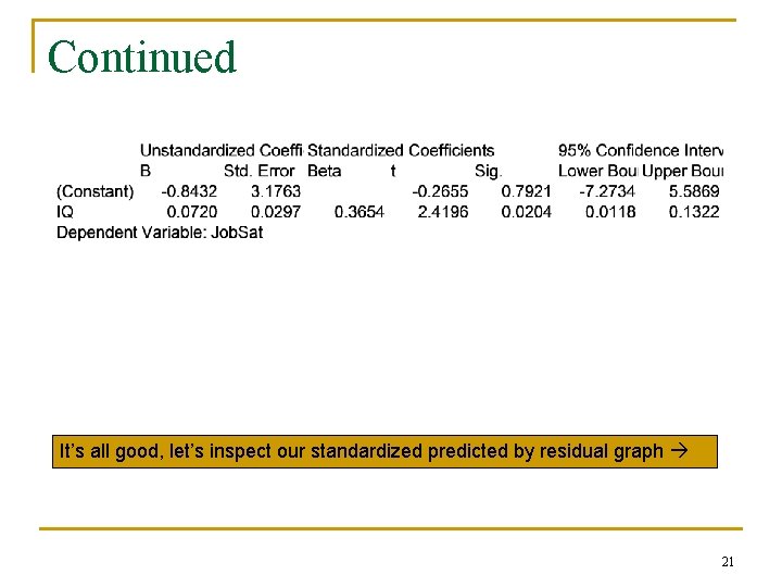
Continued It’s all good, let’s inspect our standardized predicted by residual graph 21

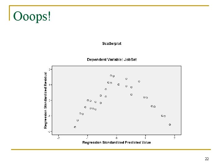
Ooops! 22

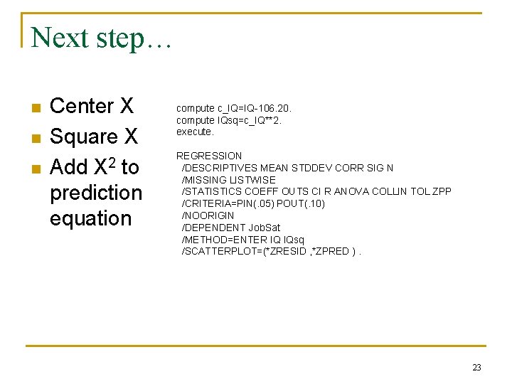
Next step… n n n Center X Square X Add X 2 to prediction equation compute c_IQ=IQ-106. 20. compute IQsq=c_IQ**2. execute. REGRESSION /DESCRIPTIVES MEAN STDDEV CORR SIG N /MISSING LISTWISE /STATISTICS COEFF OUTS CI R ANOVA COLLIN TOL ZPP /CRITERIA=PIN(. 05) POUT(. 10) /NOORIGIN /DEPENDENT Job. Sat /METHOD=ENTER IQ IQsq /SCATTERPLOT=(*ZRESID , *ZPRED ). 23

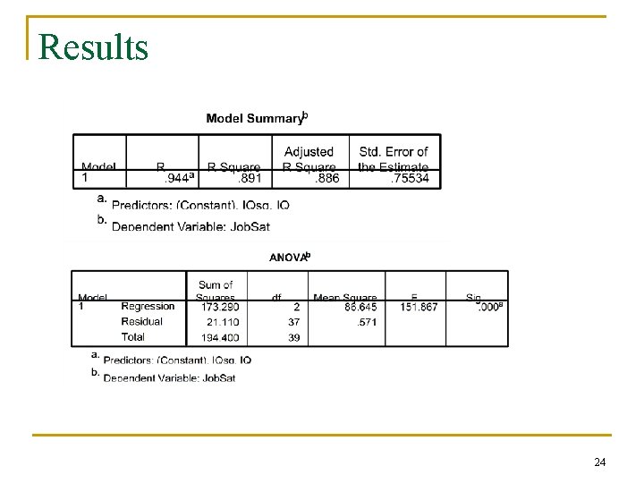
Results 24

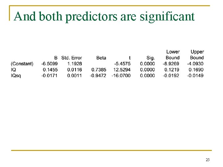
And both predictors are significant 25

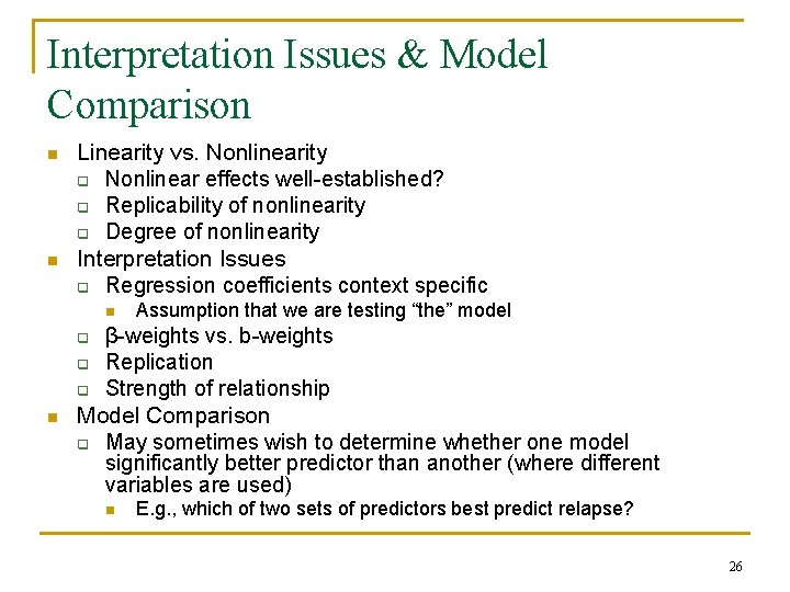
Interpretation Issues & Model Comparison n n Linearity vs. Nonlinearity q Nonlinear effects well-established? q Replicability of nonlinearity q Degree of nonlinearity Interpretation Issues q Regression coefficients context specific n q q q n Assumption that we are testing “the” model β-weights vs. b-weights Replication Strength of relationship Model Comparison q May sometimes wish to determine whether one model significantly better predictor than another (where different variables are used) n E. g. , which of two sets of predictors best predict relapse? 26

Strength of relationship: My test is sooo valid! 27