MPEG4 AVC H 264 Introduction The H 264

MPEG-4 AVC (H. 264)

Introduction The H. 264 is aimed at very low bit rate, realtime, low end-to-end delay, and mobile applications such as conversational services and internet video. n Enhanced visual quality at very low bit rates and particularly at rate below 24 kb/s. n

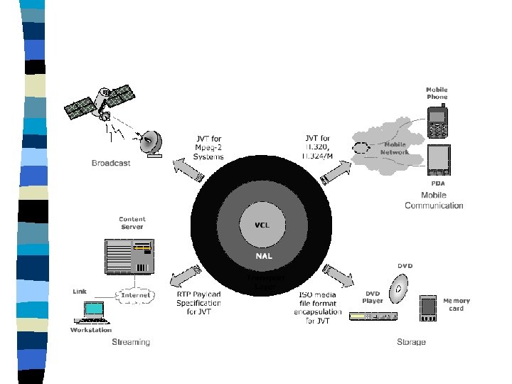
Structure of H. 264/AVC Video Coder VCL: Designed to efficiently represent the video content n NAL: formats the VCL representation of the video and provides head information for conveyance by a variety of transport layers or storage media. n

Video Coding Layer

Basic Structure of VCL Input Video Signal Coder Control Transform/ Scal. /Quant. Split into Macroblocks 16 x 16 pixels Control Data Decoder Quant. Transf. coeffs Scaling & Inv. Transform Entropy Coding Intra-frame Prediction Intra/Inter Motion. Compensation Motion Estimation De-blocking Filter Output Video Signal Motion Data

Intra-frame Prediction Input Video Signal Coder Control Transform/ Scal. /Quant. Split into Macroblocks 16 x 16 pixels Control Data Decoder Quant. Transf. coeffs Scaling & Inv. Transform Entropy Coding Intra-frame Prediction Intra/Inter Motion. Compensation Motion Estimation De-blocking Filter Output Video Signal Motion Data

n Intra-frame encoding of H. 264 supports Intra_4 4, Intra_16 16 and I_PCM. n I_PCM allows the encoder directly send the values of encoded sample. 4 and Intra_16 16 allows the intra prediction. n Intra_4

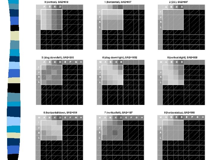
n Intra 4 4 – 9 modes – Used in texture area n Intra 16 16 – 4 modes – Used in flat area

n Four modes of Intra_16 16 – Mode 0 (vertical) : extrapolation from upper samples(H) – Mode 1 (horizontal): extrapolation from left samples(V) – Mode 2 (DC): mean of upper and left-hand samples (H+V) – Mode 3 (Plane) : a linear “plane” function is fitted to the upper and left-hand samples H and V. This works well in areas of smoothly-varying luminance

Example: Original image

n Nine modes of Intra_4 4 – The prediction block P is calculated based on the samples labeled A-M. – The encoder may select the prediction mode for each block that minimizes the residual between P and the block to be encoded

Example: Consider a 4 4 block and its neighbors labeled below. Suppose we use the mode 4 for prediction. Then a = (A + 2 M + I + 2)/4

Example:

Motion Estimation/Compensation Input Video Signal Coder Control Transform/ Scal. /Quant. Split into Macroblocks 16 x 16 pixels Control Data Decoder Quant. Transf. coeffs Scaling & Inv. Transform Entropy Coding Intra-frame Prediction Intra/Inter Motion. Compensation Motion Estimation De-blocking Filter Output Video Signal Motion Data

n Features of the H. 264 motion estimation – Various block sizes – ¼ sample accuracy • 6 -tap filtering to ½ sample accuracy • simplified filtering to ¼ sample accuracy – Multiple reference pictures – Generalized B-Frames

n Variable Block Size Block-Matching – In the H. 264, a video frame is first splitted using fixed size macroblocks. – Each macroblock may then be segmented into subblocks with different block sizes. – A macroblock has a dimension of 16 pixels. The size of the smallest subblock is 4 4 16 x 16 MB Types 0 8 x 8 Types 0 16 x 8 0 1 8 x 4 0 1 8 x 16 0 1 4 x 8 0 1 8 x 8 0 1 2 3 4 x 4 0 1 2 3

Example: This example shows the effectiveness of block matching operations with smaller sizes. Frame 1

Frame 2

Difference between Frame 1 and Frame 2

Results of block-matching operation with size 16× 16

Results of block-matching operation with size 8× 8

Results of block-matching operation with size 4× 4

To use a subblock with size less than 8 8, it is necessary to first split the macroblock into four 8 8 subblocks.

Example:

Encoding a motion vector for each subblock can cost a significant number of bits, especially if small block sizes are chosen. Motion vectors for neighboring subblocks are often highly correlated and so each motion vector is predicted from vectors of nearby, previously coded subblocks. The difference between the motion vector of the current block and its prediction is encoded and transmitted.

The method of forming the prediction depends on the block size and on the availability of nearby vectors. Let E be the current block, let A be the subblock immediately to the left of E, let B be the subblock immediately above E, and let C be the subblock above and to the right of E. It is not necessary that A, B, C, and E have the same size. C D B A E

There are two modes for the prediction of motion vectors: • Median prediction Use for all block sizes excluding 16× 8 and 8× 16 • Directional segmentation prediction Use for 16× 8 and 8× 16

C D B A E Median prediction If C not exist then C=D If B, C not exist then prediction = VA If A, C not exist then prediction = VB If A, B not exist then prediction = VC Otherwise Prediction = median(VA, , VB, VC)

Directional segmentation prediction • Vector block size 8× 16 Left: prediction = VA Right: prediction = VC • Vector block size 16× 8 Up: prediction = VB Down: prediction =VA

n Fractional Motion Estimation In H. 264, the motion vectors between current block and candidate block has ¼-pel resolution. The samples at sub-pel positions do not exist in the reference frame and so it is necessary to create them using interpolation from nearby image samples.

Interpolation of ½-pel samples. b=round((E-5 F+20 G+20 H-5 I+J)/32) h=round((A-5 C+20 G+20 M-5 R+T)/32) j=round((aa-5 bb+20 s-5 gg+hh)/32)

Interpolation of ¼-pel samples. a=round((G+b)/2) d=round((G+h)/2) e=round((b+h)/2)

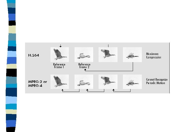
n Multiple Reference Frames

The motion estimation techniques based on multiple reference frame technique provides opportunities for more precise inter-prediction, and also improved robustness to lost picture data. The drawback of multiple reference frames is that both the encoder and decoder have to store the reference frames used for Inter-frame prediction in a multi-frame buffer.

PSNR Y [d. B] 38 37 36 35 34 33 32 31 30 29 28 27 26 0 Mobile & Calendar (CIF, 30 fps) ~15% PBB. . . with generalized B pictures PBB. . . with classic B pictures PPP. . . with 5 previous references PPP. . . with 1 previous reference 1 2 R [Mbit/s] 3 4

n Generalized B Frames Basic B-frames: The basic B-frames cannot be used as reference frames.

Generalized B-frames: The generalized B-frames can be used as reference frames.

PSNR Y [d. B] 38 37 36 35 34 33 32 31 30 29 28 27 26 0 Mobile & Calendar (CIF, 30 fps) >25% PBB. . . with generalized B pictures PBB. . . with classic B pictures PPP. . . with 5 previous references PPP. . . with 1 previous reference 1 2 R [Mbit/s] 3 4

PSNR Y [d. B] 38 37 36 35 34 33 32 31 30 29 28 27 26 0 Mobile & Calendar (CIF, 30 fps) ~40% PBB. . . with generalized B pictures PBB. . . with classic B pictures PPP. . . with 5 previous references PPP. . . with 1 previous reference 1 2 R [Mbit/s] 3 4

Transformation/Quantization Input Video Signal Coder Control Transform/ Scal. /Quant. Split into Macroblocks 16 x 16 pixels Control Data Decoder Quant. Transf. coeffs Scaling & Inv. Transform Entropy Coding Intra-frame Prediction Intra/Inter Motion. Compensation Motion Estimation De-blocking Filter Output Video Signal Motion Data

n Transformation The Discrete Cosine transform (DCT) operates on x, a block of N×N samples and creates X, and N×N block of coefficients. The forward DCT: The reverse DCT:

The elements of A are: where That is,

Example: The transform matrix A for a 4× 4 DCT is:

That is, or where

The H. 264 transform is based on the 4× 4 DCT but with some fundamental differences: 1. It is an integer transfer, . 2. The core part of the transform can be implemented using only additions and shifts. 3. A scaling multiplication is integrated into the quantizer, reducing the total number of multiplications.

Recall that where

Post-scaling (where d = c/b) 1. We call (Cx. CT) the core 2 D transform. 2. E is a matrix of scaling factors. 3. indicates that each element of (Cx. CT) is multiplies by the scaling factor in the same position in matrix E (i. e. , is scalar multiplication rather than matrix multiplication)

To simplify the implementation of the transform, d is approximated by 0. 5. In order to ensure that the transform remains orthogonal, b also needs to be modified so that:

The final forward transform becomes

The inverse transform is given by: Pre-Scaling

n Quantization H. 264 assumes a scalar quantization. The quantization should satisfy the following requirements: (a) avoid division and/or floating point arithmetic (b) incorporate the post and pre-scaling matrices Ef and Ei.

The basic forward quantizer operation is Z(u, v)= round( X(u, v)/QStep ) where X(u, v) is a transform coefficient, Z(u, v) is a quantized coefficient, and QStep is a quantizer step size.

There are 52 quantizers (i. e. , Quantization Parameter (QP)=0 -51). Increase of 1 in QP means an increase of QStep by approximately 12% Increase of 6 in QP means an increase of QStep by a factor of 2.

• Post-Scaling The post-scaling factor (PF) (i. e. , a 2 , ab/2 or b 2/4) is incorporated into the forward quantizer in the following way: 1. The input block x is transformed to give a block of unscaled coefficients W=Cf x. Cf. T. 2. Then, each coefficient in W is quantized and scaled in a single operation: Z(u, v)= round( W(u, v)×PF /QStep ) where PF is a 2 , ab/2 or b 2/4 depending on the position (u, v). Why?

In order to simplify the arithmetic, the factor (PF/QStep) is implemented as a multiplication by a factor MF and a right shift, avoiding any division operations. Z(u, v)= round( W(u, v)×MF /2 qbits ) where and qbits=15+ QP/6

Note that the round operation does not have to be the nearest integer operation. In the reference model software, the round operation is realized by |Z(u, v)|=(|W(u, v)|×MF+f)>>qbits sign(Z(u, v))=sign(W(u, v)) where f is 2 qbits/3 for Intra blocks and 2 qbits /6 for Inter blocks.

Example: Suppose QP=4 and (u, v)=(0, 0). Therefore, QStep=1. 0, PF=a 2=0. 25, and qbits=15. From We have MF=8192

The MF value for various QPs (QP 5) are shown below. Table_for_MF For QP>5, the factors MF remain unchanged, but qbits increases by 1 for each increment of six in QP. That is, qbits=16 for 6 QP 11, qbits=17 for 12 QP 17, and so on.

• Pre-Scaling The de-quantized coefficient is given by The inverse transform involving pre-scaling operations proceeds in the following way: 1. The dequantized block is pre-scaled to block for core 2 D inverse transform. 2. The reconstructed block is then given by

The pre-scaling factor (PF) (i. e. , a 2 , ab or b 2) is incorporated in the computation of , together with a constant scaling factor of 64 to avoid rounding errors. The values at the output of the inverse transform should be divided by 64 to remove the constant scaling factor.

The H. 264 standard does not specify QStep or PF directly. Instead, the parameters V=QStep×PF× 64 is defined. The V values for various QPs (QP 5) are shown below. Table_for_V

For QP>5, the V value increases by a factor of 2 for each increment of six in QP. That is, where

n The Complete Transformation, Quantization, Rescaling and Inverse Transformation Encoding: 1. Input 4× 4 block: x 2. Forward core transform: W=Cf x. Cf. T 3. Post-scaling and quantization: Z(u, v)= round( W(u, v)×MF /2 qbits ) Decoding: 1. Pre-scaling: 2. Inverse core transform: 3. Re-scaling:

Example: 1. Suppose QP=10, and input block x = 5 11 8 10 9 8 4 12 1 10 11 4 19 6 7 15 2. Forward core transform: W = 140 -1 -6 7 -19 -39 7 -92 22 17 8 31 -27 -32 -59 -21

3. MF=8192, 3355 or 5243, qbits=16 and f is 2 qbits/3. Z= 17 0 -1 -2 0 -5 3 1 1 2 -2 -1 -5 -1 4. V=32, 50 or 40 because 2 QP/6 =2. 544 0 -32 0 -40 100 0 250 96 40 32 80 -50 200 -50

5. Output of the inverse core transform after division by 64 is 4 13 8 10 8 8 4 12 1 10 10 3 18 5 7 14

Entropy Coding Input Video Signal Coder Control Transform/ Scal. /Quant. Split into Macroblocks 16 x 16 pixels Control Data Decoder Quant. Transf. coeffs Scaling & Inv. Transform Entropy Coding Intra-frame Prediction Intra/Inter Motion. Compensation Motion Estimation De-blocking Filter Output Video Signal Motion Data

Here we present two basic variable length coding (VLC) techniques used by H. 264: the Exp-Golomb code and context adaptive VLC (CAVLC). Exp-Golomb code is used universally for all symbols except for transform coefficients. CAVLC is used for coding of transform coefficients. • No end-of-block, but number of coefficients is decoded. • Coefficients are scanned backward. • Contexts are built dependent on transform coefficients.

n Exp-Golomb codes are variable length codes with a regular construction. First 9 codewords of Exp-Golomb codes

Each codeword of Exp-Golomb codes is constructed as follows: [M zeros][1][INFO] where INFO is an M-bit field carrying information. Therefore, the length of a codeword is 2 M+1.

Given a code_num, the corresponding Exp-Golomb codeword can be obtained by the following procedure: (a) M= log 2[code_num+1]) (b) INFO=code_num+1 -2 M Example: code_num=6 M= log 2[6+1]) =2 INFO=6+1 -22=3 The corresponding Exp-Golomb codeword =[M zeros][1][INFO]=00111

Given a Exp-Golomb codeword, its code_num can be found as follows: (a) Read in M leading zeros followed by 1. (b) Read M-bit INFO field (c) code_num=2 M+INFO-1 Example: Exp-Golomb codeword=00111 (a) M=2 (b) INFO=3 (c) code_num=22+3 -1=6

A parameter v to be encoded is mapped to code_num in one of 3 ways: ue(v) : Unsigned direct mapping, code_num=v. (Mainly used for macroblock type and reference frame index) se(v): Signed mapping. v is mapped to code_num as follows. code_num=2|v|, (v 0) code_num=2 v-1, (v>0) (Mainly used for motion vector difference and delta QP)

me(v): Mapped symbols. Parameter v is mapped to code_num according to a table specified in the standard. This mapping is used for coded_block_pattern parameters. An example of such a mapping is shown below.

n CAVLC This is the method used to encode residual and zig-zag ordered blocks of transform coefficients.

The CAVLC is designed to take advantage of several characteristics of quantized 4× 4 blocks: • After prediction, transformation and quantization, blocks are typically sparse (containing mostly zeros). • The highest non-zero coefficients after the zig/zag are often sequences of +/- 1. • The number of non-zero coefficients in neighboring blocks is correlated. • The level (magnitude) of non-zero coefficients tends to be higher at the start of the zig-zag scan, and lower towards the high frequencies.

The procedure described below is based on the document entitled JVT Document JVT-C 028, Gisle Bjøntegaard and Karl Lillevold, “Context-adaptive VLC (CVLC) coding of coefficients, ” Fairfax, VA, May 2002. The H. 264 CAVLC is an extension of this work.

The CAVLC encoding of a block of transform coefficients proceeds as follows. 1. 2. 3. 4. Encode the number of coefficients and trailing ones. Encode the sign of each trailing ones. Encode the levels of the remaining no-zero coefficients. Encode the total number of zeros before the last coefficients. 5. Encode each run of zeros.

• Encode the number of coefficients and trailing ones The first step is to encode the number of coefficients (Num. Coef) and trailling ones (T 1 s). Num. Coef can be anything from 0 (no coefficient in the block) to 16 (16 non-zero coefficients). T 1 s can be anything from 0 to 3. If there are more than 3 trailing +/- 1 s, only the last 3 are treated as ``special cases” and the others are coded as normal coefficients.

Example: Consider the 4× 4 block shown below -2 4 0 -1 3 0 0 0 1 0 -1 1 0 0 The Num-Coef=7, and T 1 s=3

Three tables can be used for the encoding of Num_Coeff and T 1: Num-VLC 0, Num-VLC 1 and Num-VLC 2. Num-VLC 0

The selection of tables depends on the number of non-zero coefficients in upper and left-hand previously coded blocks NU and NL. A parameter N is calculate as follows: If blocks U and L are available (i. e. , in the same coded slice), N=(NU+NL)/2 If only block U is available, N=NU. If only block L is available, N= NL. If neither is available, N=0.

The selection of table is based on N in the following way: N Selected Table 0, 1 Num-VLC 0 2, 3 Num-VLC 1 4, 5, 6, 7 Num-VLC 2 8 or above FLC The FLC is of the following form: xxxxyy (i. e. , 6 bits) where xxxx and yy represent Num_Coeff and T 1, respectively.

• Encode the sign of each trailing ones For each T 1, a single bit encodes the sign (0=+, 1=-). These are encoded in reverse order, starting with the highest frequency T 1.

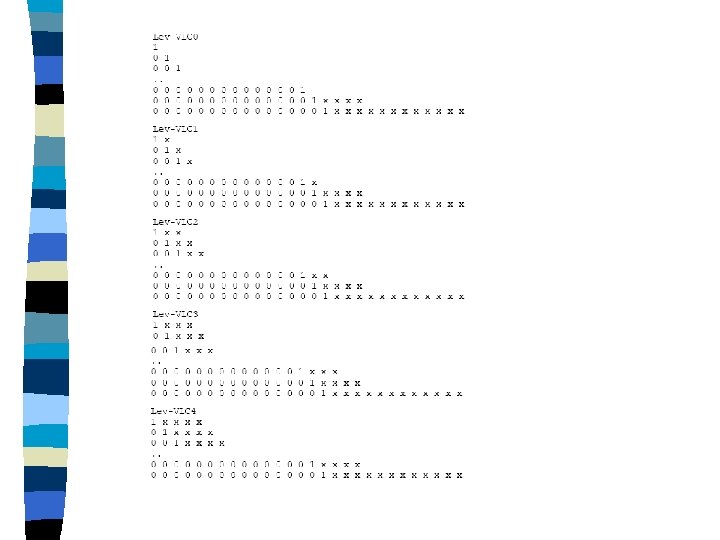
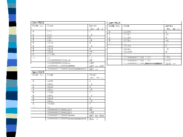
• Encode the levels of the remaining no-zero coefficients The level (sign and magnitude) of each remaining non-zero coefficient in the block is encoded in reverse order. There are 5 VLC tables to choose from, Lev_VLC 0 to Lev_VLC 4. Lev_VLC 0 is biased towards lower magnitudes; Lev_VLC 1 is biased towards slightly higher magnitudes, and so on.

This is used only when it is impossible for a coefficient to have values +/- 1. It will happen when T 1 s<3.

To improve coding efficiency, the tables are changed along with the coding process based on the following procedure.

• Encode the total number of zeros before the last coefficient The following shows the table for encoding the total number of zeros before the last coefficient (Tot. Zeros)

• Encode each run of zeros At this stage it is known how many zeros are left to distribute (call this Zeros. Left). When encoding or decoding a non-zero coefficient for the first time, Zeros. Left begins at Tot. Zeros, and decreases as more non-zero coefficients are encoded or decoded. The number of preceding zeros before each non-zero coefficient (called Run. Before) needs to be coded to properly locate that coefficient. Before coding the next Run. Before, Zeros. Left is updated and used to select one out of 7 tables.

zero-left Why the maximum number is 14?

Example: Consider the following interframe residual 4× 4 block 0 3 -1 0 0 -1 1 0 0 0 0 The zigzag re-ordering of the block is shown below: 0, 3, 0, 1, -1, 0, 0, 0 Therefore, Num. Coeff=5, Tot. Zero=3, T 1 s=3 Assume N=0

Encoding: Value Code Comments Num. Coeff=5, T 1 s=3 0001011 Use Num-VLC 0 sign of T 1 (1) 0 Starting at highest frequency sign of T 1(-1) 1 Level= +1 1 Use Lev-VLC 0 Level= +3 0010 Use Lev-VLC 1 Tot. Zeros=3 1110 Also depends on Num. Coeff Zeros. Left=3; Run. Before=1 00 Run. Before of the 1 st Coeff Zeros. Left=2; Run. Before=0 1 Run. Before of the 2 nd Coeff Zeros. Left=2; Run. Before=0 1 Run. Before of the 3 rd Coeff Zeros. Left=2; Run. Before=1 01 Run. Before of the 4 th Coeff Zeros. Left=1; Run. Before=1 No code required; last coeff The transmitted bitstream for this block is 000101101110001101

Decoding: Code Value Output Array Comments 0001011 Num. Coeff=5, T 1 s=3 Empty 0 + 1 T 1 sign 1 - -1, -1, 1 T 1 sign 1 +1 1, -1, 1 level value 0010 +3 +3, 1, -1, 1 level value 1110 Tot. Zeros=3 +3, 1, -1, 1 00 Run. Before=1 +3, 1, -1, 0, 1 Run. Before of the 1 st Coeff 1 Run. Before=0 +3, 1, -1, 0, 1 Run. Before of the 2 nd Coeff 1 Run. Before=0 +3, 1, -1, 0, 1 Run. Before of the 3 rd Coeff 01 Run. Before=1 +3, 0, 1, -1, 0, 1 Run. Before of the 4 th Coeff 0, +3, 0, 1, -1, 0, 1 Zero. Left=1

De-block Filter Input Video Signal Coder Control Transform/ Scal. /Quant. Split into Macroblocks 16 x 16 pixels Control Data Decoder Quant. Transf. coeffs Scaling & Inv. Transform Entropy Coding Intra-frame Prediction Intra/Inter Motion. Compensation Motion Estimation De-blocking Filter Output Video Signal Motion Data

The beblocking filter improves subjective visual quality. The filter is highly context adaptive. It operates on the boundary of 4× 4 subblock as shown below. q 3 q 2 q 1 q 0 p 0 p 1 p 2 p 3

The choice of filtering outcome depends on the boundary strength and on the gradient of image samples across the boundary. The boundary strength parameter Bs is selected according to the following rules.

A group of samples from the set (p 2, p 1, p 0, q 1, q 2) is filtered only if: (a) Bs>0 and (b) |p 0 -q 0| < and |p 1 -p 0| < and |q 1 -q 0| < where and are thresholds defined in the standard. The threshold values increase with the average quantizer parameter QP of two blocks q and p.

When QP is small, anything other than a very small gradient across the boundary is likely to be due to image features that should be preserved and so the thresholds and are low. When QP is larger, blocking distortion is likely to be more significant and are higher so that more boundary samples are filtered.

without deblock filtering with deblock filtering

Data Partitioning and Network Abstraction Layer

A video picture is coded as one or more slices. Each slice contains an integral number of macroblocks from 1 to total number of macroblocks in a picture. The number of macroblocks per slice need not to be constant within a picture.

There are five slice modes. Three commonly use modes are: 1. I-slice: A slice where all macroblocks of the slice are coded using intra prediction. 2. P-slice: In addition to the coding types of the Islice, some macroblocks of the P-slice can be coded using inter-prediction (predicted from one reference picture buffer only). 3. B-slice: In addition to the coding types available in a P-slice, some macroblocks of the B-slice can be predicted from two reference picture buffers.

Note that the coded data in a slice can be placed in three separate Data Partitions (A, B and C) for robust transmission. Partition A contains the slice header and header data for each marcoblock in the slice. Partition B contains coded residual data for Intra slice macroblocks. Partition C contains coded residual data for Inter slice macroblocks.

In the H. 264, the VCL data will be mapped into NAL units prior to transmission or storage. Each NAL unit contains a Raw Byte Sequence Payload (RBSP), a set of data corresponding to coded video data or header information. The NAL units can be delivered over a packet-based network or a bitstream transmission link or stored in a file. NAL header RBSP NAL header sequence of NAL units RBSP NAL header RBSP

RBSP type Description Parameter Set Global parameter for a sequence such as picture dimensions, video format. Supplemental Enhancement Information Side messages that are not essential for correct decoding of the video sequences. Picture Delimiter Boundary between pictures (optional). If not present, the decoder infers the boundary based on the frame number contained within each slice header. Coded Slice Header and data for a slice; this RBSP contains actual coded video data. Data Partition A, B or C Three units containing Data Partitioned slice layer data (useful for error decoding). End of Sequence End of Stream Filler Data Contains ‘dummy’ data

Example: The following figure shows an example of RBSP elements. Sequence parameter set SEI Picture parameter set I Slice (Coded slice) Picture delimiter P Slice (Coded slice) . . .

Profiles n Baseline n Main n Extended n High