Machine Learning for Signal Processing Prediction and Estimation

Machine Learning for Signal Processing Prediction and Estimation, Part II Bhiksha Raj Class 24. 21 Nov 2013 11 -755/18797 1

Administrivia • HW 1 scores out – Some students (who got really poor marks) given chance to upgrade • Make it all the way to the 50 percentile for each problem • HW 2 scores to be out by next week • Please send us project updates 21 Nov 2013 11 -755/18797 2

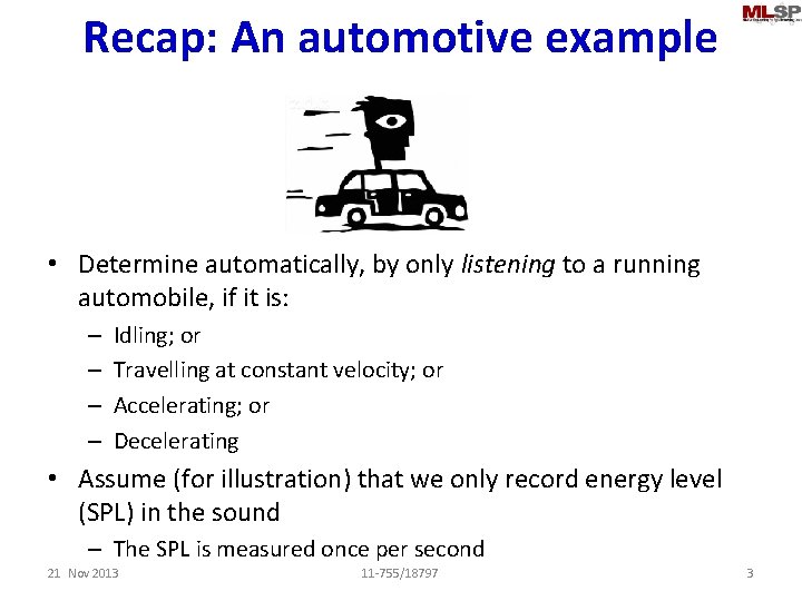
Recap: An automotive example • Determine automatically, by only listening to a running automobile, if it is: – – Idling; or Travelling at constant velocity; or Accelerating; or Decelerating • Assume (for illustration) that we only record energy level (SPL) in the sound – The SPL is measured once per second 21 Nov 2013 11 -755/18797 3

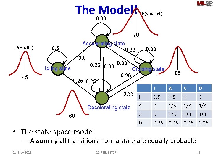
The 0. 33 Model! P(x|accel) 70 P(x|idle) Accelerating state 0. 5 Idling state 45 0. 33 0. 25 0. 33 Cruising state 65 0. 25 0. 33 Decelerating state 60 I A C D I 0. 5 0 0 A 0 1/3 1/3 C 0 1/3 1/3 D 0. 25 • The state-space model – Assuming all transitions from a state are equally probable 21 Nov 2013 11 -755/18797 4

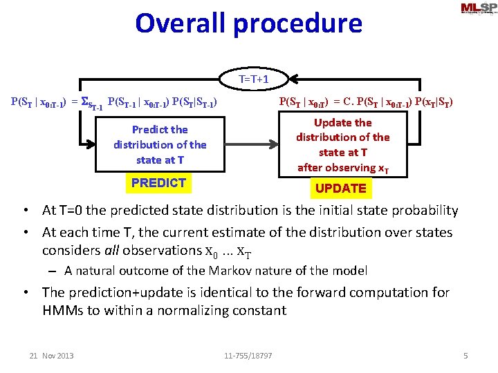
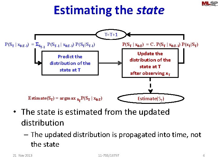
Overall procedure T=T+1 P(ST | x 0: T-1) = SST-1 P(ST-1 | x 0: T-1) P(ST|ST-1) P(ST | x 0: T) = C. P(ST | x 0: T-1) P(x. T|ST) Update the distribution of the state at T after observing x. T Predict the distribution of the state at T PREDICT UPDATE • At T=0 the predicted state distribution is the initial state probability • At each time T, the current estimate of the distribution over states considers all observations x 0. . . x. T – A natural outcome of the Markov nature of the model • The prediction+update is identical to the forward computation for HMMs to within a normalizing constant 21 Nov 2013 11 -755/18797 5

Estimating the state T=T+1 P(ST | x 0: T-1) = SST-1 P(ST-1 | x 0: T-1) P(ST|ST-1) P(ST | x 0: T) = C. P(ST | x 0: T-1) P(x. T|ST) Update the distribution of the state at T after observing x. T Predict the distribution of the state at T Estimate(ST) = argmax STP(ST | x 0: T) Estimate(ST) • The state is estimated from the updated distribution – The updated distribution is propagated into time, not the state 21 Nov 2013 11 -755/18797 6

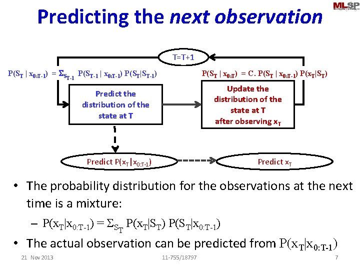
Predicting the next observation T=T+1 P(ST | x 0: T-1) = SST-1 P(ST-1 | x 0: T-1) P(ST|ST-1) P(ST | x 0: T) = C. P(ST | x 0: T-1) P(x. T|ST) Update the distribution of the state at T after observing x. T Predict the distribution of the state at T Predict P(x. T|x 0: T-1) Predict x. T • The probability distribution for the observations at the next time is a mixture: – P(x. T|x 0: T-1) = SST P(x. T|ST) P(ST|x 0: T-1) • The actual observation can be predicted from P(x. T|x 0: T-1) 21 Nov 2013 11 -755/18797 7

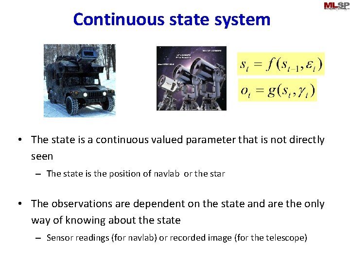
Continuous state system • The state is a continuous valued parameter that is not directly seen – The state is the position of navlab or the star • The observations are dependent on the state and are the only way of knowing about the state – Sensor readings (for navlab) or recorded image (for the telescope)

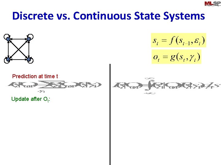
Discrete vs. Continuous State Systems 1 2 0 3 Prediction at time t: Update after Ot:

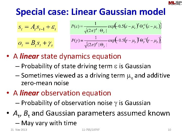
Special case: Linear Gaussian model • A linear state dynamics equation – Probability of state driving term e is Gaussian – Sometimes viewed as a driving term me and additive zero-mean noise • A linear observation equation – Probability of observation noise g is Gaussian • At, Bt and Gaussian parameters assumed known – May vary with time 21 Nov 2013 11 -755/18797 10

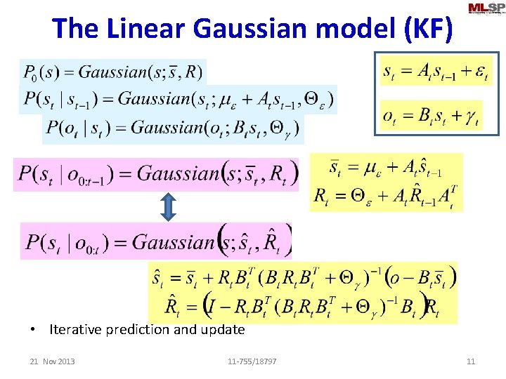
The Linear Gaussian model (KF) • Iterative prediction and update 21 Nov 2013 11 -755/18797 11

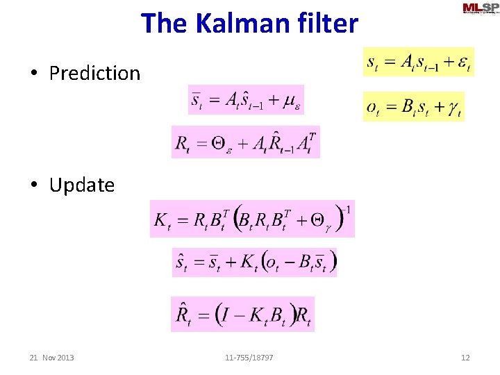
The Kalman filter • Prediction • Update 21 Nov 2013 11 -755/18797 12

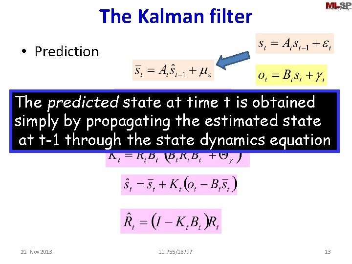
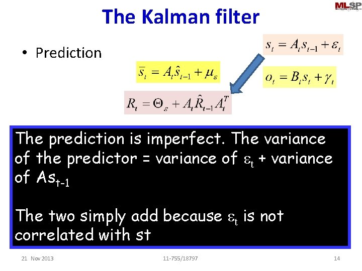
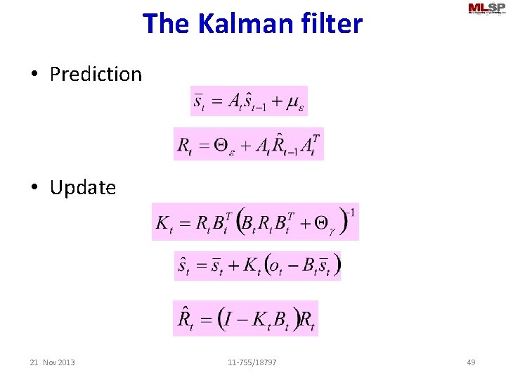
The Kalman filter • Prediction The predicted state at time t is obtained simply by propagating the estimated state • Update at t-1 through the state dynamics equation 21 Nov 2013 11 -755/18797 13

The Kalman filter • Prediction • Update The prediction is imperfect. The variance of the predictor = variance of et + variance of Ast-1 The two simply add because et is not correlated with st 21 Nov 2013 11 -755/18797 14

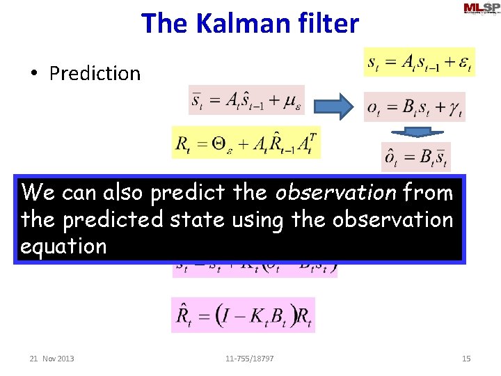
The Kalman filter • Prediction • Update We can also predict the observation from the predicted state using the observation equation 21 Nov 2013 11 -755/18797 15

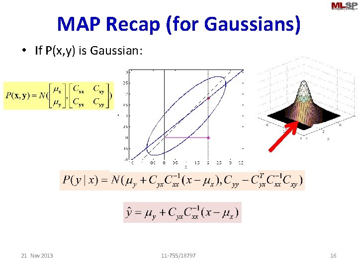
MAP Recap (for Gaussians) • If P(x, y) is Gaussian: 21 Nov 2013 11 -755/18797 16

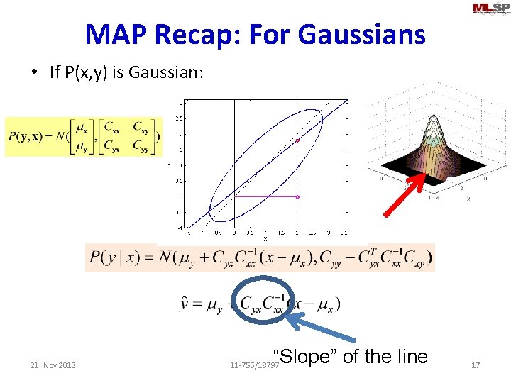
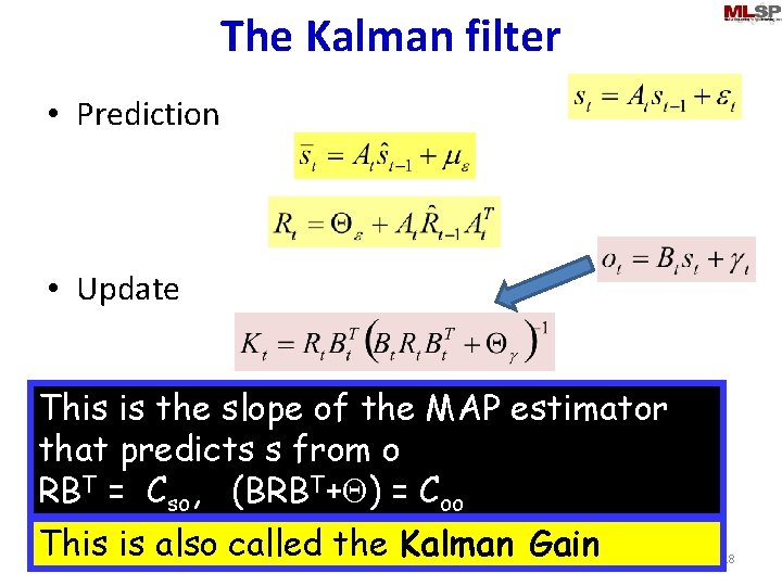
MAP Recap: For Gaussians • If P(x, y) is Gaussian: 21 Nov 2013 “Slope” of the line 11 -755/18797 17

The Kalman filter • Prediction • Update This is the slope of the MAP estimator that predicts s from o RBT = Cso, (BRBT+Q) = Coo This is also called the Kalman Gain 21 Nov 2013 11 -755/18797 18

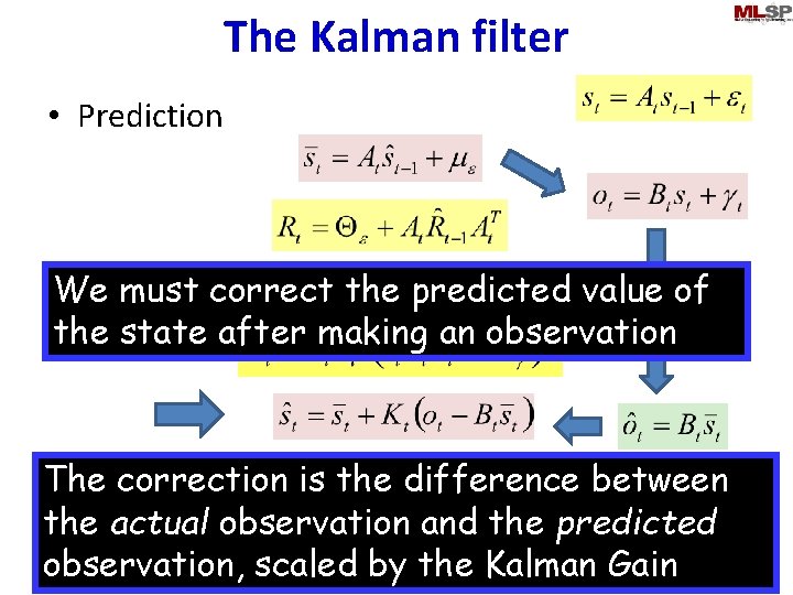
The Kalman filter • Prediction must correct the predicted value of • We Update the state after making an observation The correction is the difference between the actual observation and the predicted observation, scaled by the Kalman Gain 21 Nov 2013 11 -755/18797 19

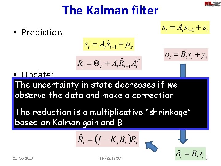
The Kalman filter • Prediction • Update: The uncertainty in state decreases if we observe the data and make a correction The reduction is a multiplicative “shrinkage” on Kalman gain and B • based Update 21 Nov 2013 11 -755/18797 20

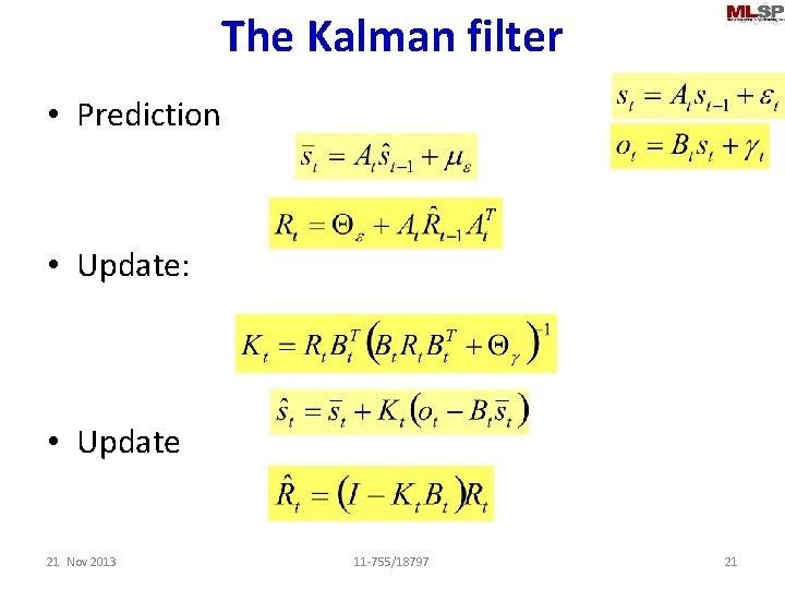
The Kalman filter • Prediction • Update: • Update 21 Nov 2013 11 -755/18797 21

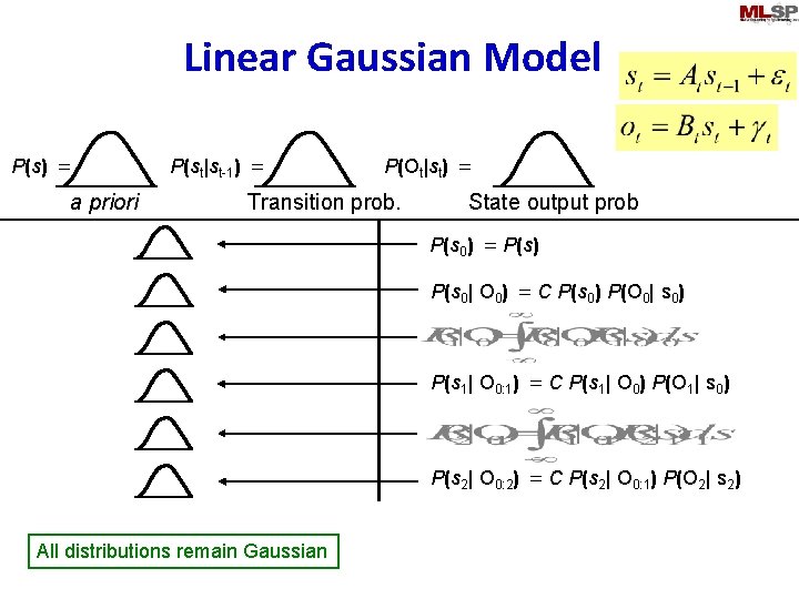
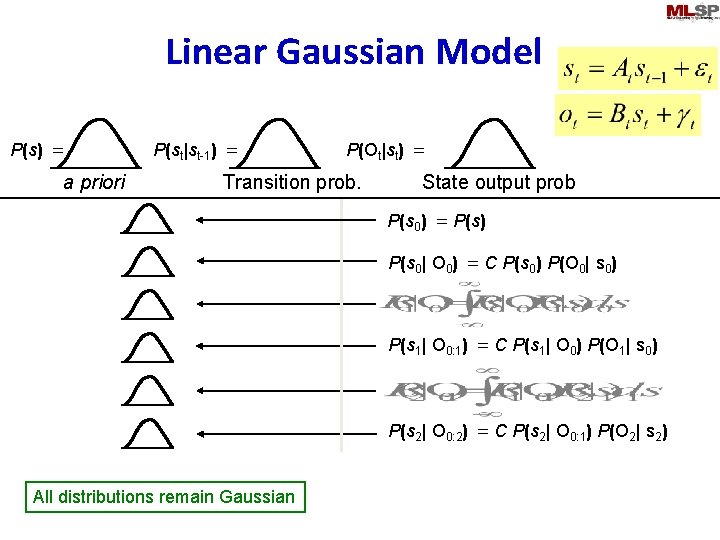
Linear Gaussian Model P(s) = a priori P(st|st-1) = P(Ot|st) = Transition prob. State output prob P(s 0) = P(s) P(s 0| O 0) = C P(s 0) P(O 0| s 0) P(s 1| O 0: 1) = C P(s 1| O 0) P(O 1| s 0) P(s 2| O 0: 2) = C P(s 2| O 0: 1) P(O 2| s 2) All distributions remain Gaussian

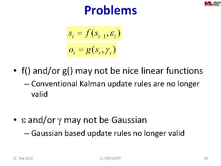
Problems • f() and/or g() may not be nice linear functions – Conventional Kalman update rules are no longer valid • e and/or g may not be Gaussian – Gaussian based update rules no longer valid 21 Nov 2013 11 -755/18797 23

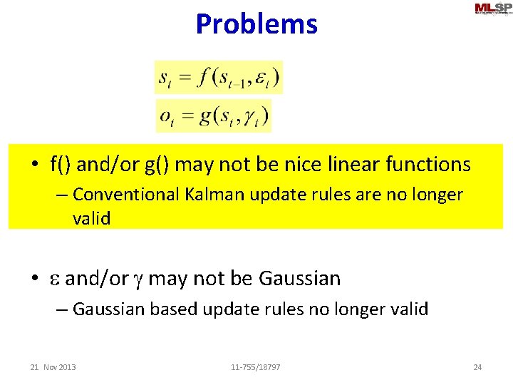
Problems • f() and/or g() may not be nice linear functions – Conventional Kalman update rules are no longer valid • e and/or g may not be Gaussian – Gaussian based update rules no longer valid 21 Nov 2013 11 -755/18797 24

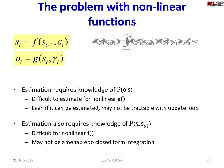
The problem with non-linear functions • Estimation requires knowledge of P(o|s) – Difficult to estimate for nonlinear g() – Even if it can be estimated, may not be tractable with update loop • Estimation also requires knowledge of P(st|st-1) – Difficult for nonlinear f() – May not be amenable to closed form integration 21 Nov 2013 11 -755/18797 25

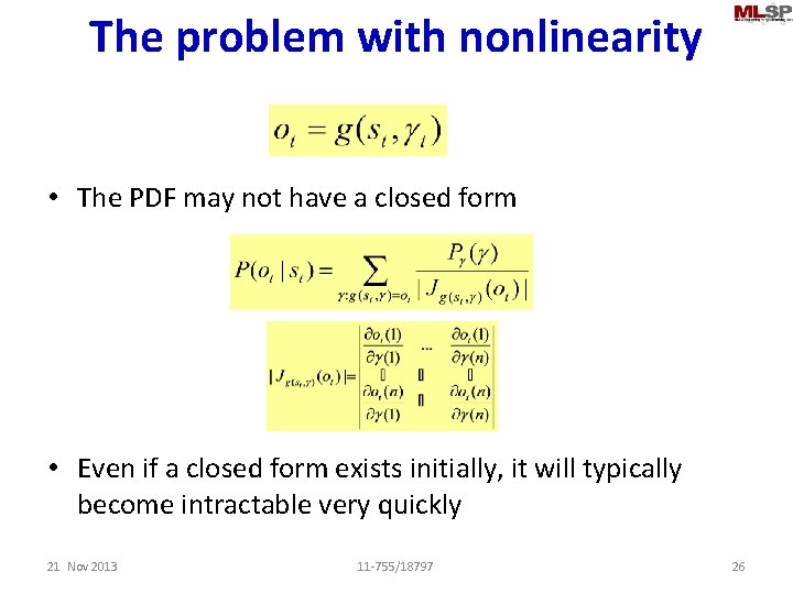
The problem with nonlinearity • The PDF may not have a closed form • Even if a closed form exists initially, it will typically become intractable very quickly 21 Nov 2013 11 -755/18797 26

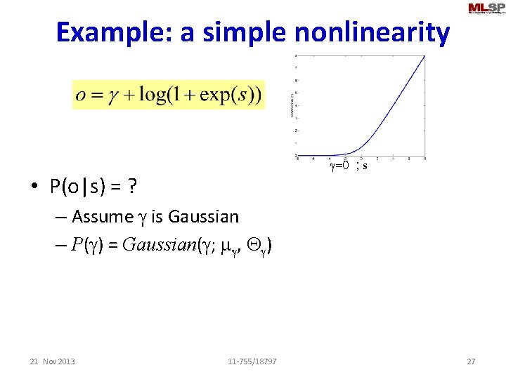
Example: a simple nonlinearity g=0 ; s • P(o|s) = ? – Assume g is Gaussian – P(g) = Gaussian(g; mg, Qg) 21 Nov 2013 11 -755/18797 27

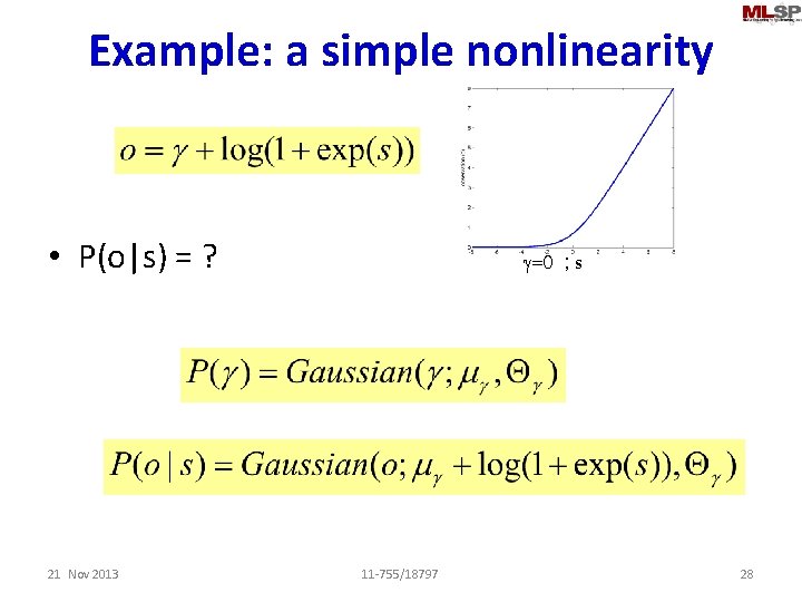
Example: a simple nonlinearity • P(o|s) = ? 21 Nov 2013 g=0 ; s 11 -755/18797 28

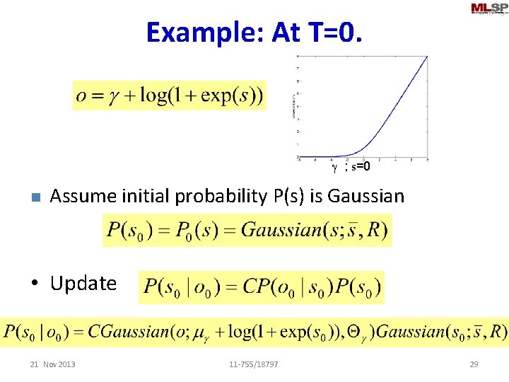
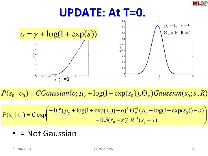
Example: At T=0. g ; s=0 n Assume initial probability P(s) is Gaussian • Update 21 Nov 2013 11 -755/18797 29

UPDATE: At T=0. g ; s=0 • = Not Gaussian 21 Nov 2013 11 -755/18797 30

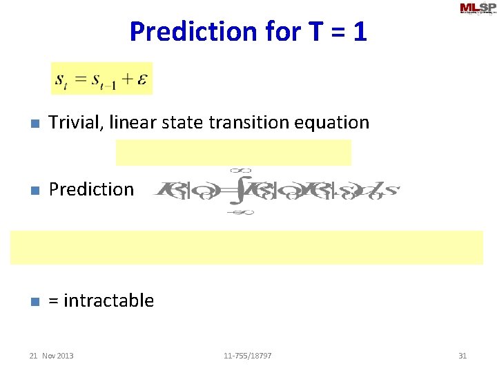
Prediction for T = 1 n Trivial, linear state transition equation n Prediction n = intractable 21 Nov 2013 11 -755/18797 31

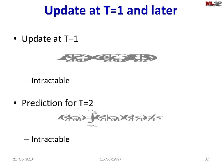
Update at T=1 and later • Update at T=1 – Intractable • Prediction for T=2 – Intractable 21 Nov 2013 11 -755/18797 32

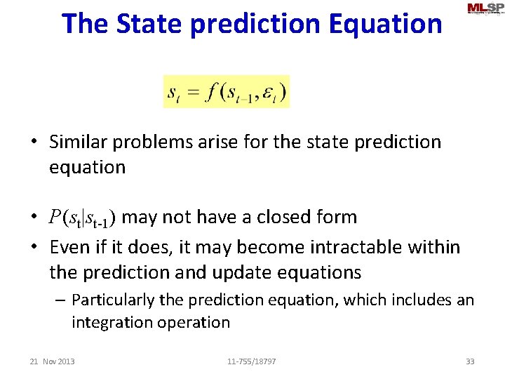
The State prediction Equation • Similar problems arise for the state prediction equation • P(st|st-1) may not have a closed form • Even if it does, it may become intractable within the prediction and update equations – Particularly the prediction equation, which includes an integration operation 21 Nov 2013 11 -755/18797 33

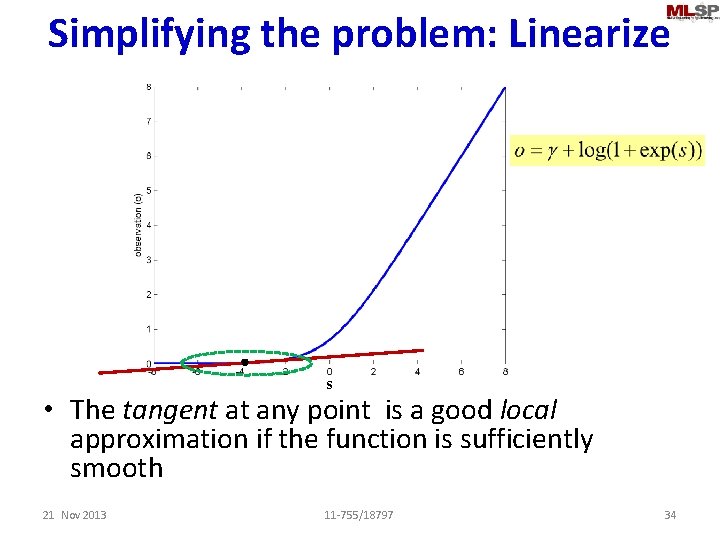
Simplifying the problem: Linearize s • The tangent at any point is a good local approximation if the function is sufficiently smooth 21 Nov 2013 11 -755/18797 34

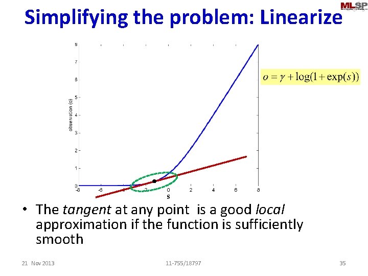
Simplifying the problem: Linearize s • The tangent at any point is a good local approximation if the function is sufficiently smooth 21 Nov 2013 11 -755/18797 35

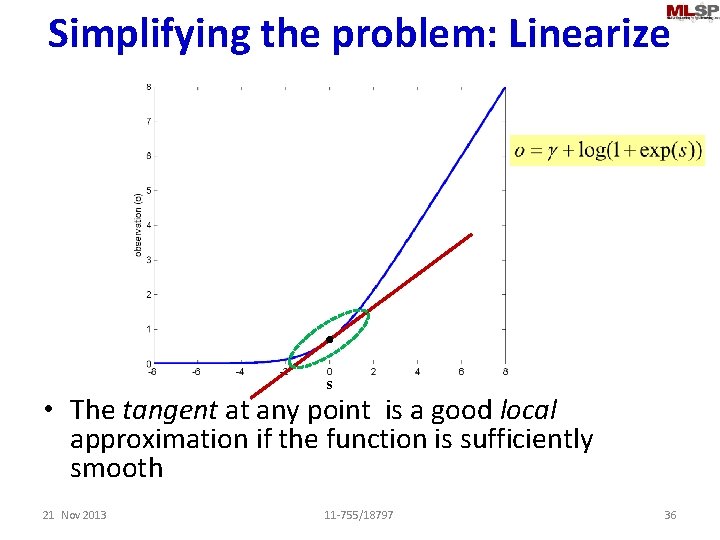
Simplifying the problem: Linearize s • The tangent at any point is a good local approximation if the function is sufficiently smooth 21 Nov 2013 11 -755/18797 36

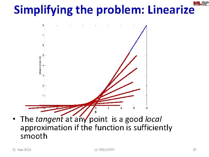
Simplifying the problem: Linearize s • The tangent at any point is a good local approximation if the function is sufficiently smooth 21 Nov 2013 11 -755/18797 37

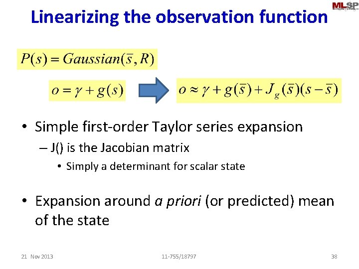
Linearizing the observation function • Simple first-order Taylor series expansion – J() is the Jacobian matrix • Simply a determinant for scalar state • Expansion around a priori (or predicted) mean of the state 21 Nov 2013 11 -755/18797 38

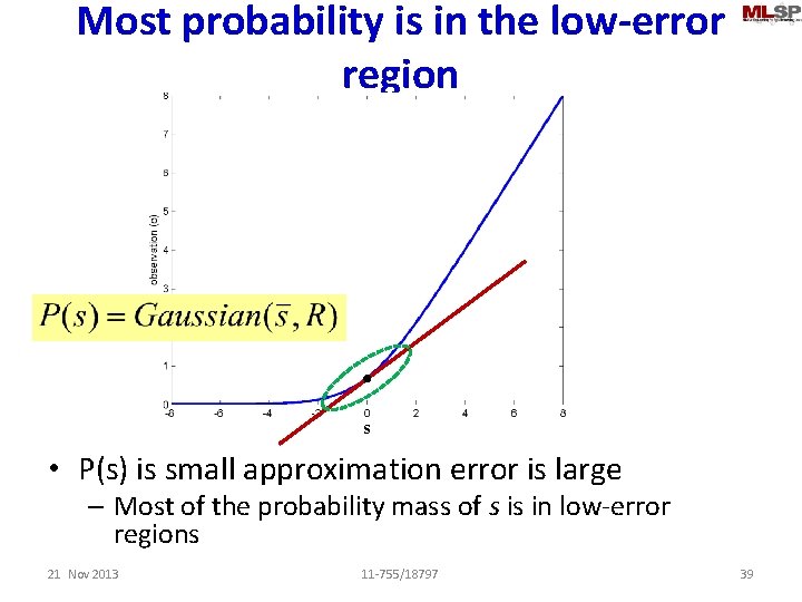
Most probability is in the low-error region s • P(s) is small approximation error is large – Most of the probability mass of s is in low-error regions 21 Nov 2013 11 -755/18797 39

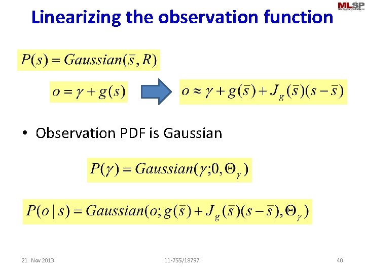
Linearizing the observation function • Observation PDF is Gaussian 21 Nov 2013 11 -755/18797 40

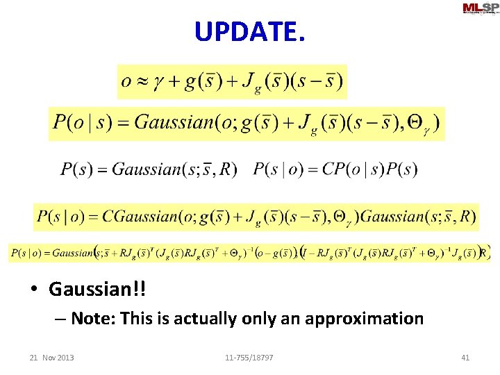
UPDATE. • Gaussian!! – Note: This is actually only an approximation 21 Nov 2013 11 -755/18797 41

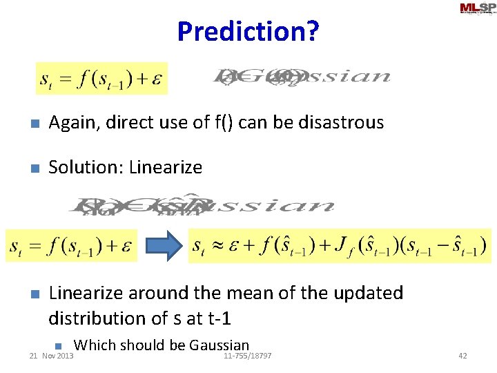
Prediction? n Again, direct use of f() can be disastrous n Solution: Linearize n Linearize around the mean of the updated distribution of s at t-1 n Which should be Gaussian 11 -755/18797 21 Nov 2013 42

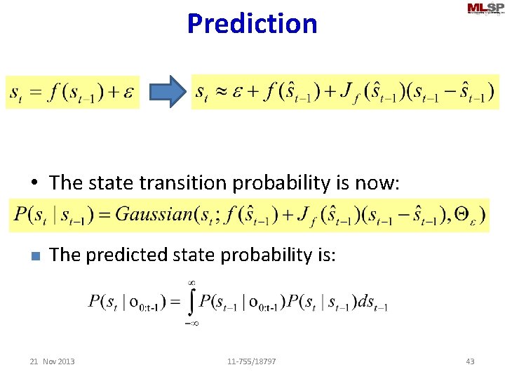
Prediction • The state transition probability is now: n The predicted state probability is: 21 Nov 2013 11 -755/18797 43

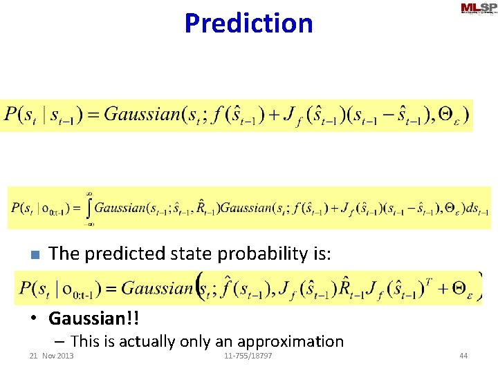
Prediction n The predicted state probability is: • Gaussian!! – This is actually only an approximation 21 Nov 2013 11 -755/18797 44

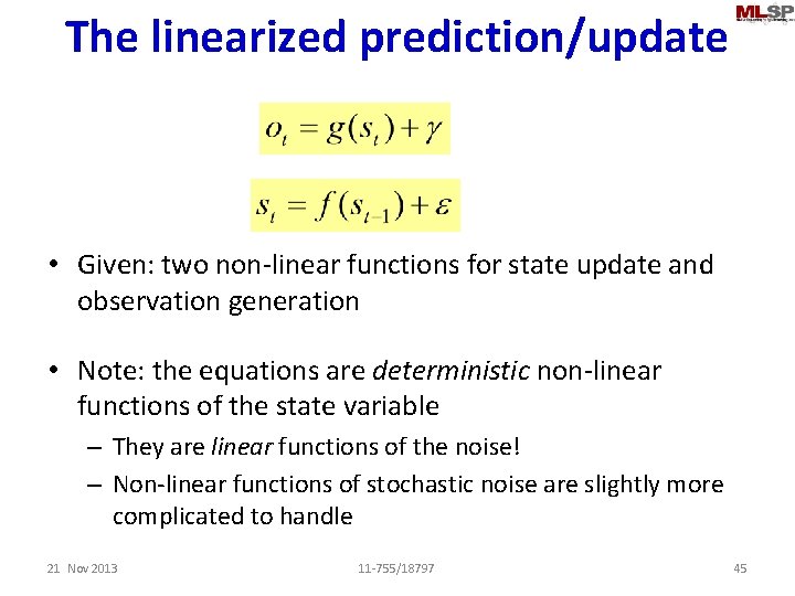
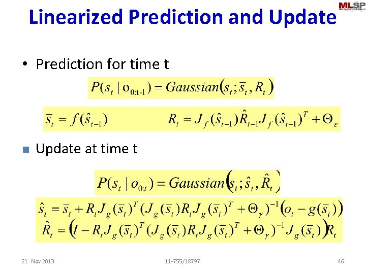
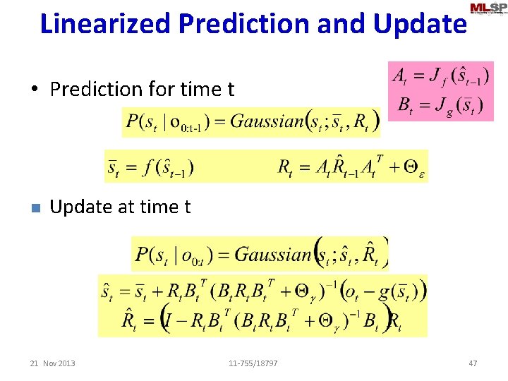
The linearized prediction/update • Given: two non-linear functions for state update and observation generation • Note: the equations are deterministic non-linear functions of the state variable – They are linear functions of the noise! – Non-linear functions of stochastic noise are slightly more complicated to handle 21 Nov 2013 11 -755/18797 45

Linearized Prediction and Update • Prediction for time t n Update at time t 21 Nov 2013 11 -755/18797 46

Linearized Prediction and Update • Prediction for time t n Update at time t 21 Nov 2013 11 -755/18797 47

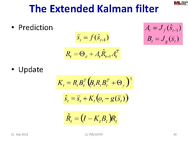
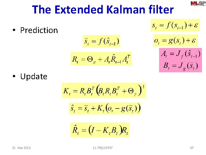
The Extended Kalman filter • Prediction • Update 21 Nov 2013 11 -755/18797 48

The Kalman filter • Prediction • Update 21 Nov 2013 11 -755/18797 49

The Extended Kalman filter • Prediction • Update 21 Nov 2013 11 -755/18797 50

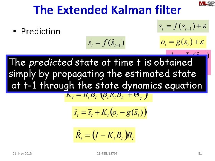
The Extended Kalman filter • Prediction The predicted state at time t is obtained simply by propagating the estimated state • Update at t-1 through the state dynamics equation 21 Nov 2013 11 -755/18797 51

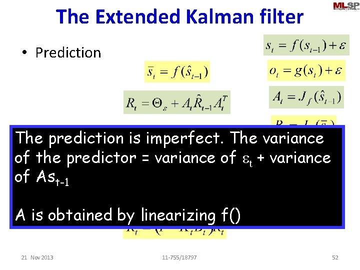
The Extended Kalman filter • Prediction • Update The prediction is imperfect. The variance of the predictor = variance of et + variance of Ast-1 A is obtained by linearizing f() 21 Nov 2013 11 -755/18797 52

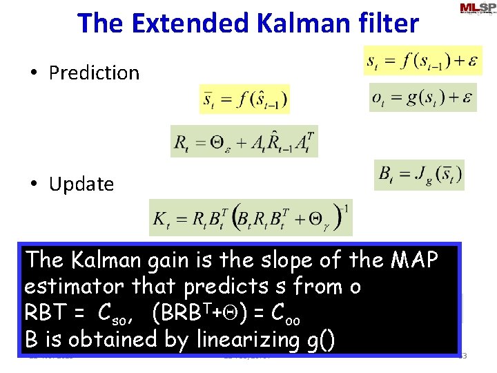
The Extended Kalman filter • Prediction • Update The Kalman gain is the slope of the MAP estimator that predicts s from o RBT = Cso, (BRBT+Q) = Coo B is obtained by linearizing g() 21 Nov 2013 11 -755/18797 53

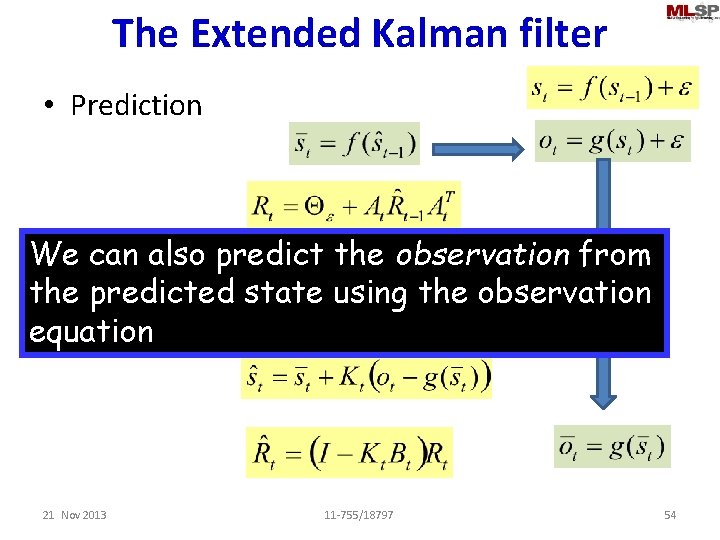
The Extended Kalman filter • Prediction We can also predict the observation from • Update the predicted state using the observation equation 21 Nov 2013 11 -755/18797 54

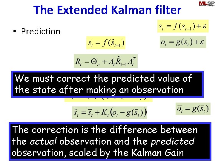
The Extended Kalman filter • Prediction must correct the predicted value of • We Update the state after making an observation The correction is the difference between the actual observation and the predicted observation, scaled by the Kalman Gain 21 Nov 2013 11 -755/18797 55

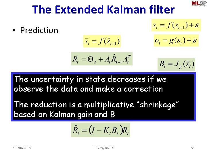
The Extended Kalman filter • Prediction • The Update uncertainty in state decreases if we observe the data and make a correction The reduction is a multiplicative “shrinkage” based on Kalman gain and B 21 Nov 2013 11 -755/18797 56

The Extended Kalman filter • Prediction • Update 21 Nov 2013 11 -755/18797 57

EKFs • EKFs are probably the most commonly used algorithm for tracking and prediction – Most systems are non-linear – Specifically, the relationship between state and observation is usually nonlinear – The approach can be extended to include non-linear functions of noise as well • The term “Kalman filter” often simply refers to an extended Kalman filter in most contexts. • But. . 21 Nov 2013 11 -755/18797 58

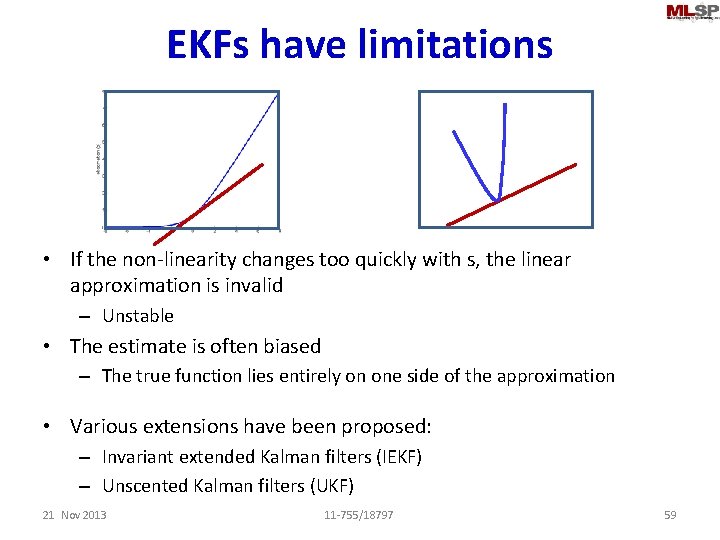
EKFs have limitations • If the non-linearity changes too quickly with s, the linear approximation is invalid – Unstable • The estimate is often biased – The true function lies entirely on one side of the approximation • Various extensions have been proposed: – Invariant extended Kalman filters (IEKF) – Unscented Kalman filters (UKF) 21 Nov 2013 11 -755/18797 59

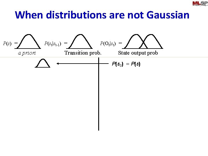
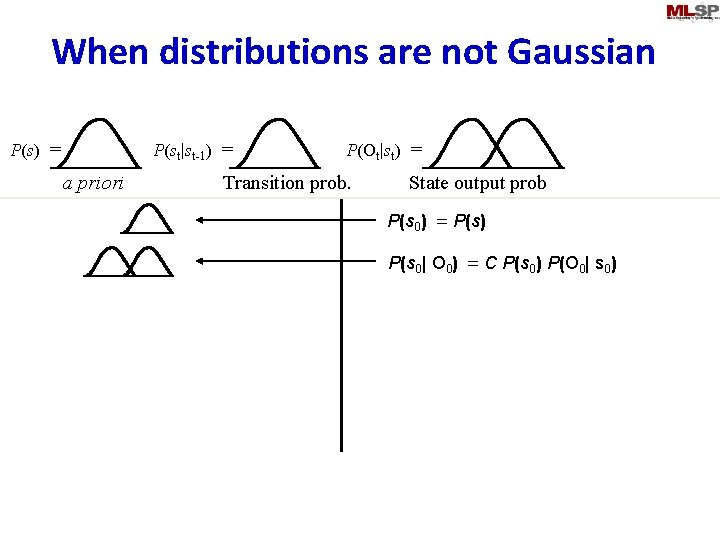
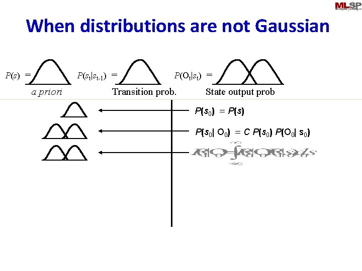
A different problem: Non-Gaussian PDFs • We have assumed so far that: – P 0(s) is Gaussian or can be approximated as Gaussian – P(e) is Gaussian – P(g) is Gaussian • This has a happy consequence: All distributions remain Gaussian • But when any of these are not Gaussian, the results are not so happy 21 Nov 2013 11 -755/18797 60

Linear Gaussian Model P(s) = a priori P(st|st-1) = P(Ot|st) = Transition prob. State output prob P(s 0) = P(s) P(s 0| O 0) = C P(s 0) P(O 0| s 0) P(s 1| O 0: 1) = C P(s 1| O 0) P(O 1| s 0) P(s 2| O 0: 2) = C P(s 2| O 0: 1) P(O 2| s 2) All distributions remain Gaussian

A different problem: Non-Gaussian PDFs • We have assumed so far that: – P 0(s) is Gaussian or can be approximated as Gaussian – P(e) is Gaussian – P(g) is Gaussian • This has a happy consequence: All distributions remain Gaussian • But when any of these are not Gaussian, the results are not so happy 21 Nov 2013 11 -755/18797 62

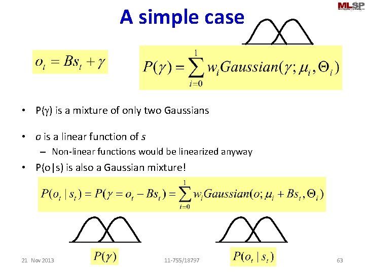
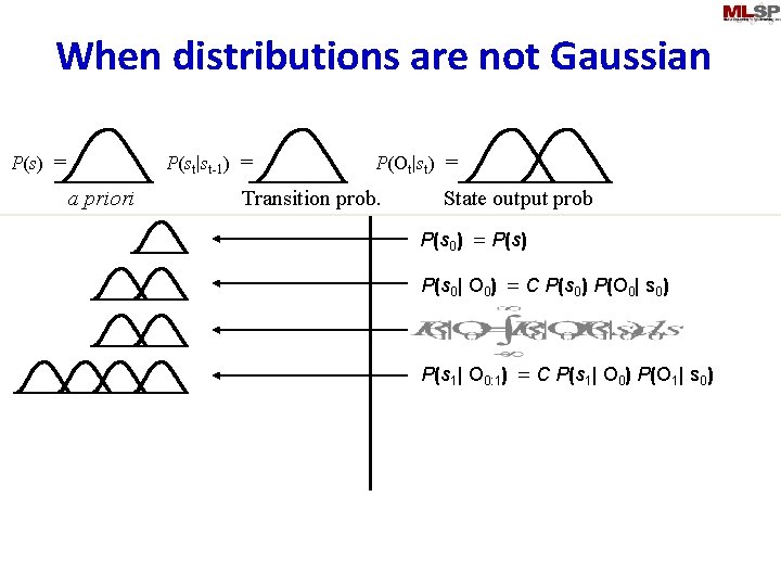
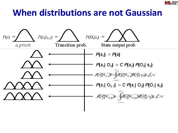
A simple case • P(g) is a mixture of only two Gaussians • o is a linear function of s – Non-linear functions would be linearized anyway • P(o|s) is also a Gaussian mixture! 21 Nov 2013 11 -755/18797 63

When distributions are not Gaussian P(st|st-1) = P(s) = a priori P(Ot|st) = Transition prob. State output prob P(s 0) = P(s)

When distributions are not Gaussian P(st|st-1) = P(s) = a priori P(Ot|st) = Transition prob. State output prob P(s 0) = P(s) P(s 0| O 0) = C P(s 0) P(O 0| s 0)

When distributions are not Gaussian P(st|st-1) = P(s) = a priori P(Ot|st) = Transition prob. State output prob P(s 0) = P(s) P(s 0| O 0) = C P(s 0) P(O 0| s 0)

When distributions are not Gaussian P(st|st-1) = P(s) = a priori P(Ot|st) = Transition prob. State output prob P(s 0) = P(s) P(s 0| O 0) = C P(s 0) P(O 0| s 0) P(s 1| O 0: 1) = C P(s 1| O 0) P(O 1| s 0)

When distributions are not Gaussian P(st|st-1) = P(s) = a priori P(Ot|st) = Transition prob. State output prob P(s 0) = P(s) P(s 0| O 0) = C P(s 0) P(O 0| s 0) P(s 1| O 0: 1) = C P(s 1| O 0) P(O 1| s 0)

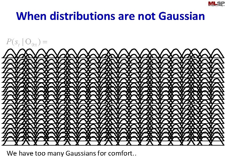
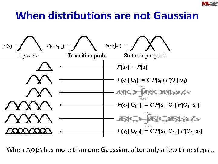
When distributions are not Gaussian P(st|st-1) = P(s) = a priori P(Ot|st) = Transition prob. State output prob P(s 0) = P(s) P(s 0| O 0) = C P(s 0) P(O 0| s 0) P(s 1| O 0: 1) = C P(s 1| O 0) P(O 1| s 0) P(s 2| O 0: 2) = C P(s 2| O 0: 1) P(O 2| s 2) When P(Ot|st) has more than one Gaussian, after only a few time steps…

When distributions are not Gaussian We have too many Gaussians for comfort. .

Related Topic: How to sample from a Distribution? • “Sampling from a Distribution P(x; G) with parameters G” • Generate random numbers such that – The distribution of a large number of generated numbers is P(x; G) – The parameters of the distribution are G • Many algorithms to generate RVs from a variety of distributions – Generation from a uniform distribution is well studied – Uniform RVs used to sample from multinomial distributions – Other distributions: Most commonly, transform a uniform RV to the desired distribution 21 Nov 2013 11 -755/18797 71

Sampling from a multinomial • Given a multinomial over N symbols, with probability of ith symbol = P(i) • Randomly generate symbols from this distribution • Can be done by sampling from a uniform distribution 21 Nov 2013 11 -755/18797 72

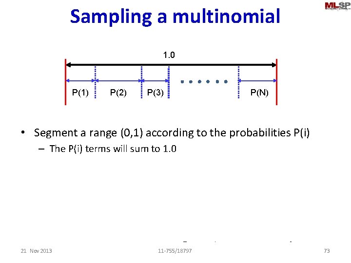
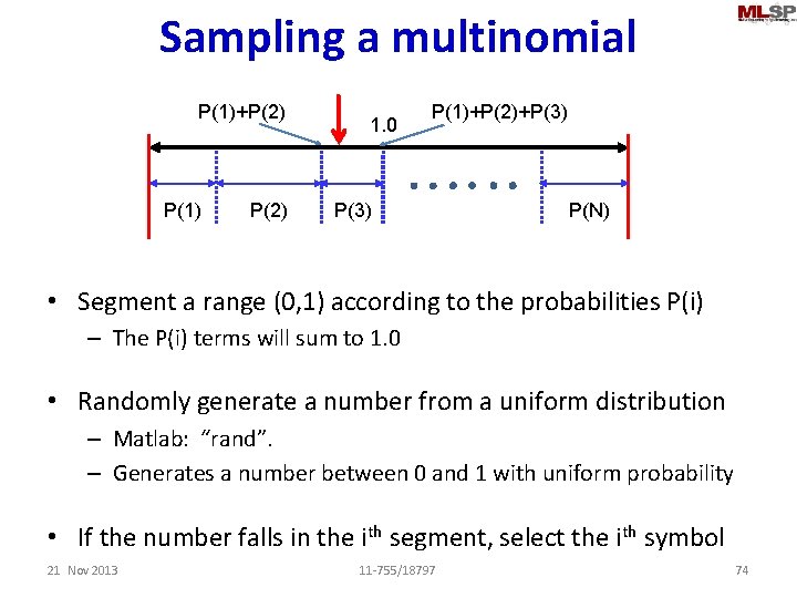
Sampling a multinomial 1. 0 P(1) P(2) P(3) P(N) • Segment a range (0, 1) according to the probabilities P(i) – The P(i) terms will sum to 1. 0 • Randomly generate a number from a uniform distribution – Matlab: “rand”. – Generates a number between 0 and 1 with uniform probability • If the number falls in the ith segment, select the ith symbol 21 Nov 2013 11 -755/18797 73

Sampling a multinomial P(1)+P(2) P(1) P(2) 1. 0 P(1)+P(2)+P(3) P(N) • Segment a range (0, 1) according to the probabilities P(i) – The P(i) terms will sum to 1. 0 • Randomly generate a number from a uniform distribution – Matlab: “rand”. – Generates a number between 0 and 1 with uniform probability • If the number falls in the ith segment, select the ith symbol 21 Nov 2013 11 -755/18797 74

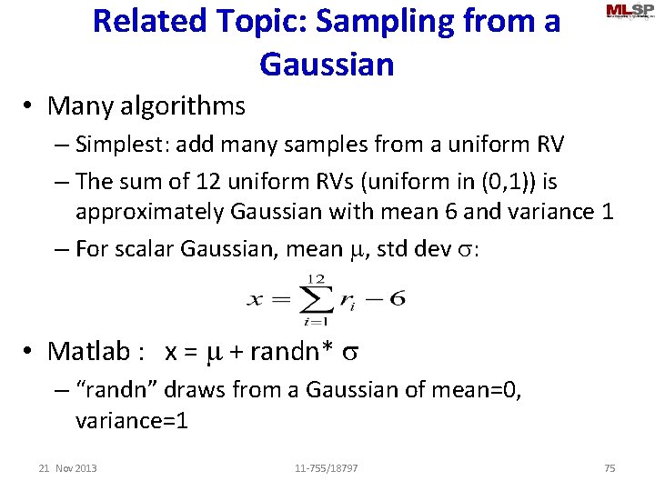
Related Topic: Sampling from a Gaussian • Many algorithms – Simplest: add many samples from a uniform RV – The sum of 12 uniform RVs (uniform in (0, 1)) is approximately Gaussian with mean 6 and variance 1 – For scalar Gaussian, mean m, std dev s: • Matlab : x = m + randn* s – “randn” draws from a Gaussian of mean=0, variance=1 21 Nov 2013 11 -755/18797 75

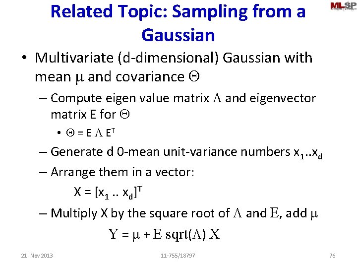
Related Topic: Sampling from a Gaussian • Multivariate (d-dimensional) Gaussian with mean m and covariance Q – Compute eigen value matrix L and eigenvector matrix E for Q • Q = E L ET – Generate d 0 -mean unit-variance numbers x 1. . xd – Arrange them in a vector: X = [x 1. . xd]T – Multiply X by the square root of L and E, add m Y = m + E sqrt(L) X 21 Nov 2013 11 -755/18797 76

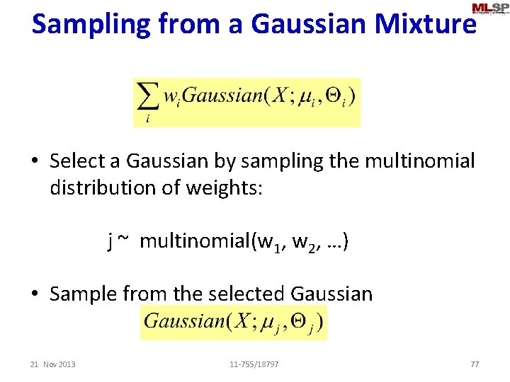
Sampling from a Gaussian Mixture • Select a Gaussian by sampling the multinomial distribution of weights: j ~ multinomial(w 1, w 2, …) • Sample from the selected Gaussian 21 Nov 2013 11 -755/18797 77

When distributions are not Gaussian P(st|st-1) = P(s) = a priori P(Ot|st) = Transition prob. State output prob P(s 0) = P(s) P(s 0| O 0) = C P(s 0) P(O 0| s 0) P(s 1| O 0: 1) = C P(s 1| O 0) P(O 1| s 0) P(s 2| O 0: 2) = C P(s 2| O 0: 1) P(O 2| s 2) When P(Ot|st) has more than one Gaussian, after only a few time steps…

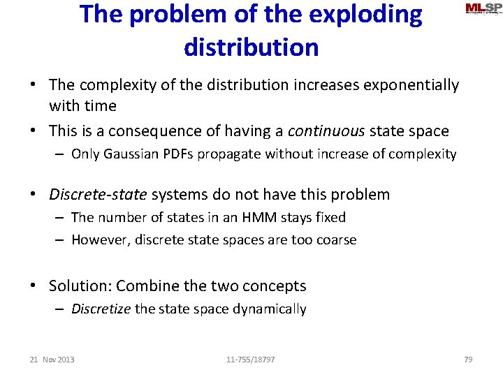
The problem of the exploding distribution • The complexity of the distribution increases exponentially with time • This is a consequence of having a continuous state space – Only Gaussian PDFs propagate without increase of complexity • Discrete-state systems do not have this problem – The number of states in an HMM stays fixed – However, discrete state spaces are too coarse • Solution: Combine the two concepts – Discretize the state space dynamically 21 Nov 2013 11 -755/18797 79

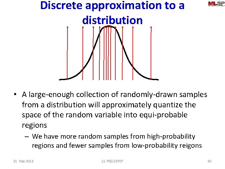
Discrete approximation to a distribution • A large-enough collection of randomly-drawn samples from a distribution will approximately quantize the space of the random variable into equi-probable regions – We have more random samples from high-probability regions and fewer samples from low-probability reigons 21 Nov 2013 11 -755/18797 80

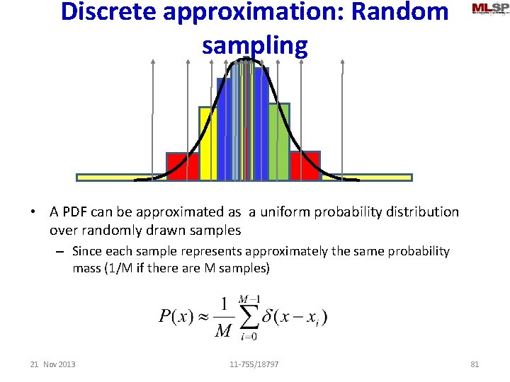
Discrete approximation: Random sampling • A PDF can be approximated as a uniform probability distribution over randomly drawn samples – Since each sample represents approximately the same probability mass (1/M if there are M samples) 21 Nov 2013 11 -755/18797 81

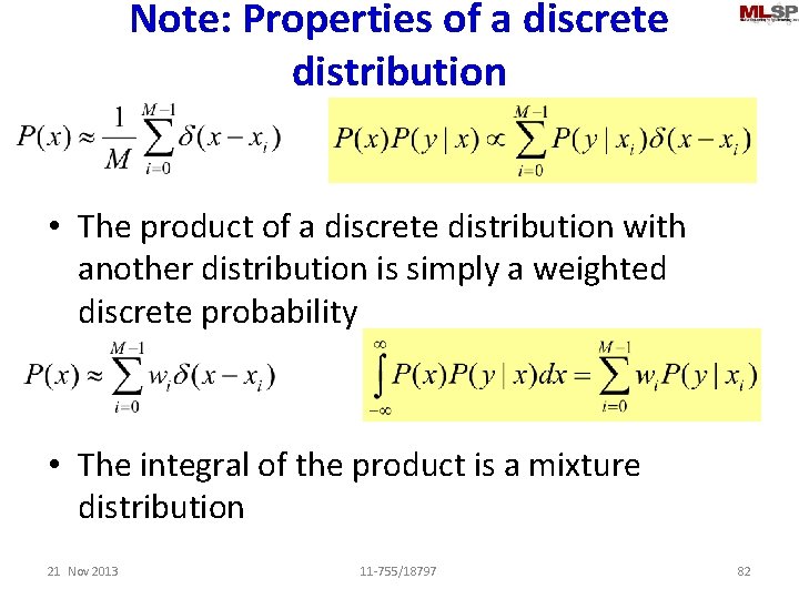
Note: Properties of a discrete distribution • The product of a discrete distribution with another distribution is simply a weighted discrete probability • The integral of the product is a mixture distribution 21 Nov 2013 11 -755/18797 82

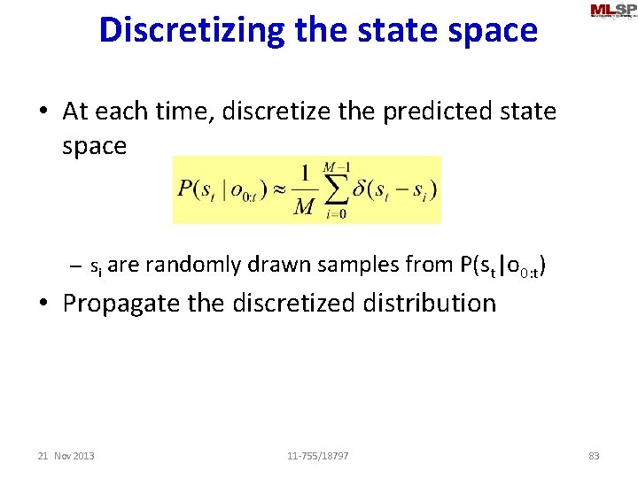
Discretizing the state space • At each time, discretize the predicted state space – si are randomly drawn samples from P(st|o 0: t) • Propagate the discretized distribution 21 Nov 2013 11 -755/18797 83

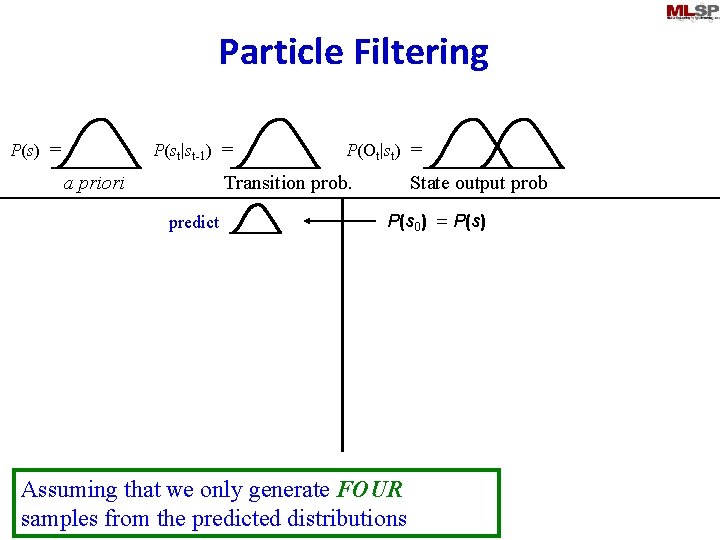
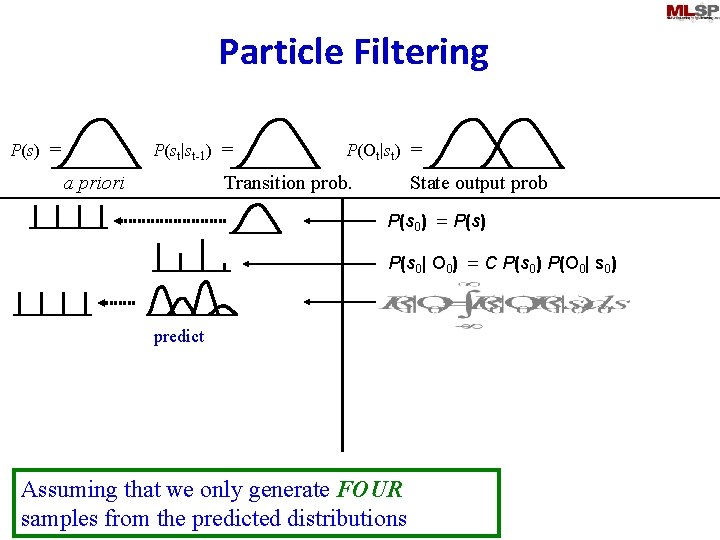
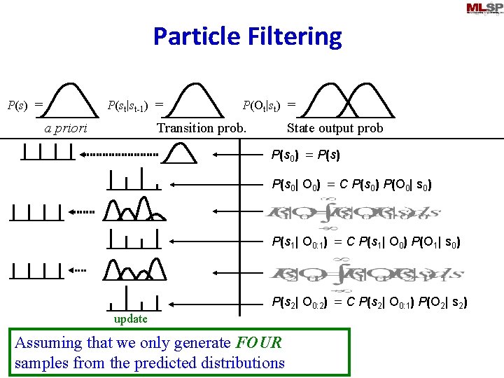
Particle Filtering P(st|st-1) = P(s) = a priori P(Ot|st) = Transition prob. predict State output prob P(s 0) = P(s) Assuming that we only generate FOUR samples from the predicted distributions

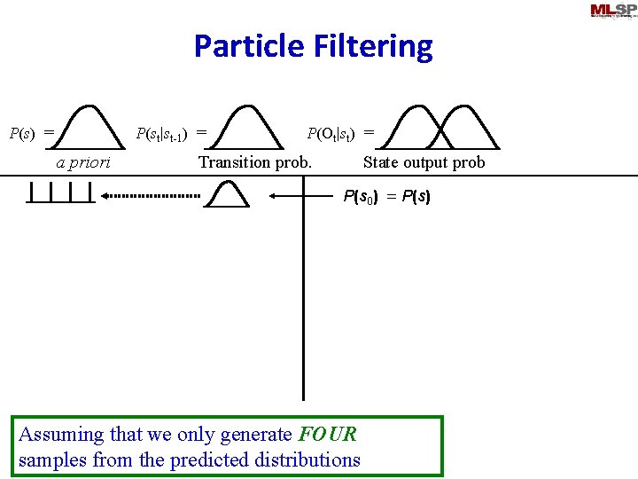
Particle Filtering P(st|st-1) = P(s) = a priori P(Ot|st) = Transition prob. State output prob P(s 0) = P(s) sample Assuming that we only generate FOUR samples from the predicted distributions

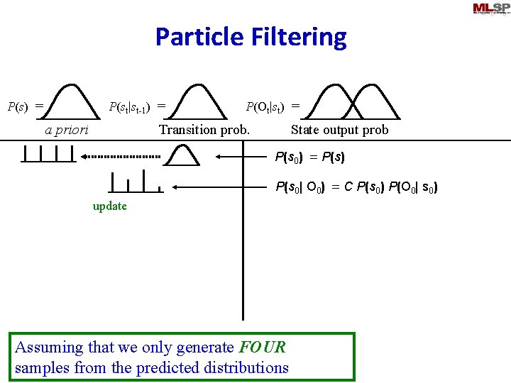
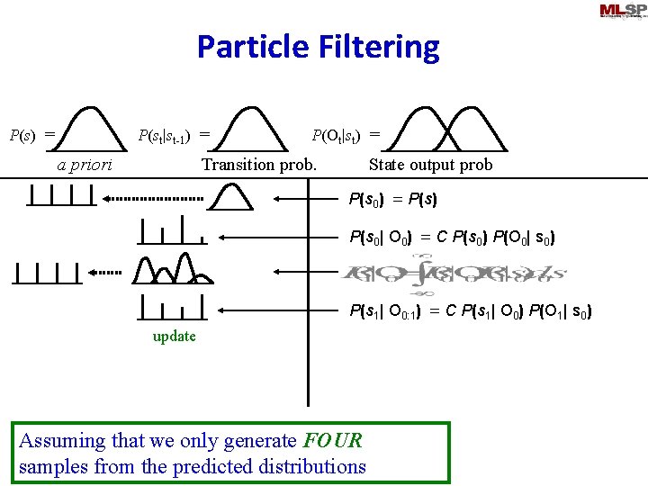
Particle Filtering P(st|st-1) = P(s) = a priori P(Ot|st) = Transition prob. State output prob P(s 0) = P(s) sample P(s 0| O 0) = C P(s 0) P(O 0| s 0) update Assuming that we only generate FOUR samples from the predicted distributions

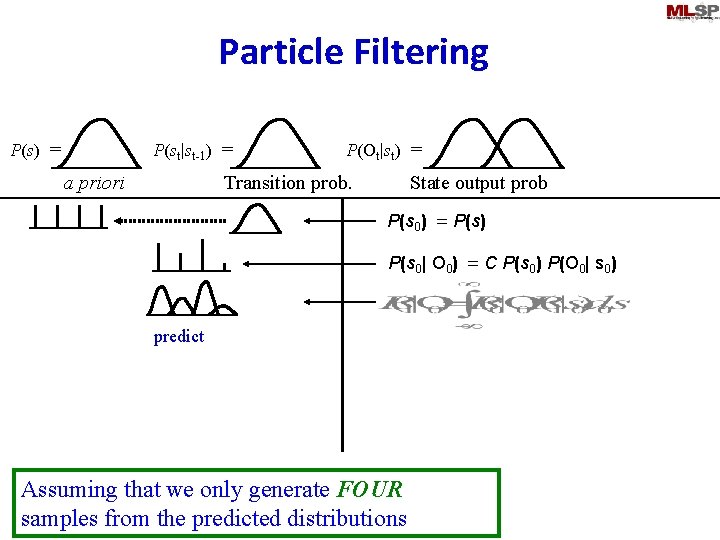
Particle Filtering P(st|st-1) = P(s) = a priori P(Ot|st) = Transition prob. State output prob P(s 0) = P(s) sample P(s 0| O 0) = C P(s 0) P(O 0| s 0) predict Assuming that we only generate FOUR samples from the predicted distributions

Particle Filtering P(st|st-1) = P(s) = a priori P(Ot|st) = Transition prob. State output prob P(s 0) = P(s) P(s 0| O 0) = C P(s 0) P(O 0| s 0) predict Assuming that we only generate FOUR samples from the predicted distributions

Particle Filtering P(st|st-1) = P(s) = a priori P(Ot|st) = Transition prob. State output prob P(s 0) = P(s) sample P(s 0| O 0) = C P(s 0) P(O 0| s 0) P(s 1| O 0: 1) = C P(s 1| O 0) P(O 1| s 0) update Assuming that we only generate FOUR samples from the predicted distributions

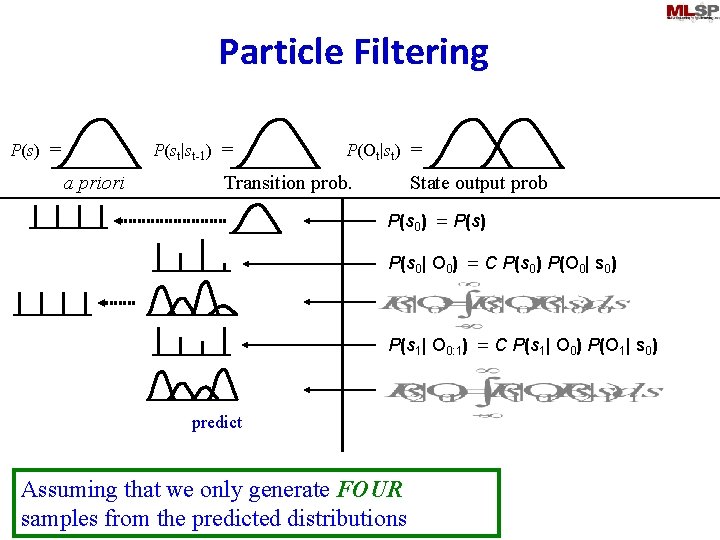
Particle Filtering P(st|st-1) = P(s) = a priori P(Ot|st) = Transition prob. State output prob P(s 0) = P(s) sample P(s 0| O 0) = C P(s 0) P(O 0| s 0) P(s 1| O 0: 1) = C P(s 1| O 0) P(O 1| s 0) predict Assuming that we only generate FOUR samples from the predicted distributions

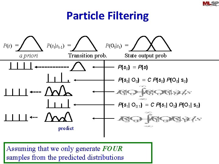
Particle Filtering P(st|st-1) = P(s) = a priori P(Ot|st) = Transition prob. State output prob P(s 0) = P(s) sample P(s 0| O 0) = C P(s 0) P(O 0| s 0) P(s 1| O 0: 1) = C P(s 1| O 0) P(O 1| s 0) predict Assuming that we only generate FOUR samples from the predicted distributions

Particle Filtering P(st|st-1) = P(s) = a priori P(Ot|st) = Transition prob. State output prob P(s 0) = P(s) sample P(s 0| O 0) = C P(s 0) P(O 0| s 0) P(s 1| O 0: 1) = C P(s 1| O 0) P(O 1| s 0) P(s 2| O 0: 2) = C P(s 2| O 0: 1) P(O 2| s 2) update Assuming that we only generate FOUR samples from the predicted distributions

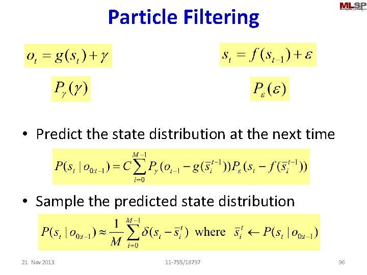
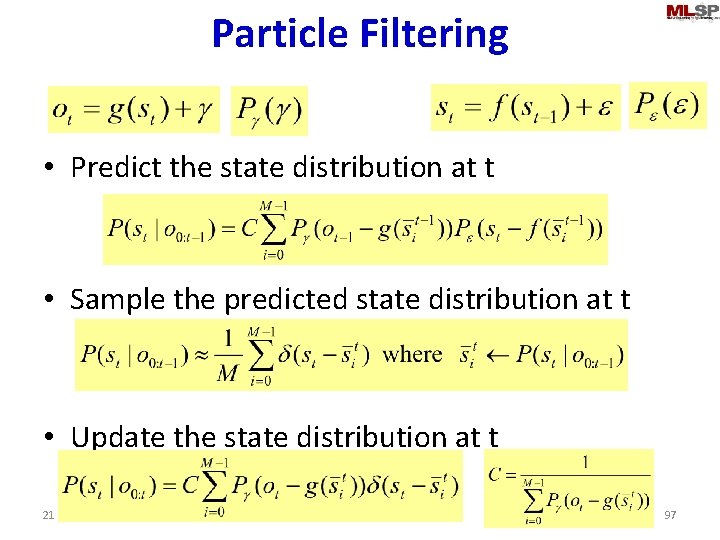
Particle Filtering • Discretize state space at the prediction step – By sampling the continuous predicted distribution • If appropriately sampled, all generated samples may be considered to be equally probable – Sampling results in a discrete uniform distribution • Update step updates the distribution of the quantized state space – Results in a discrete non-uniform distribution • Predicted state distribution for the next time instant will again be continuous – Must be discretized again by sampling • At any step, the current state distribution will not have more components than the number of samples generated at the previous sampling step – The complexity of distributions remains constant 21 Nov 2013 11 -755/18797 93

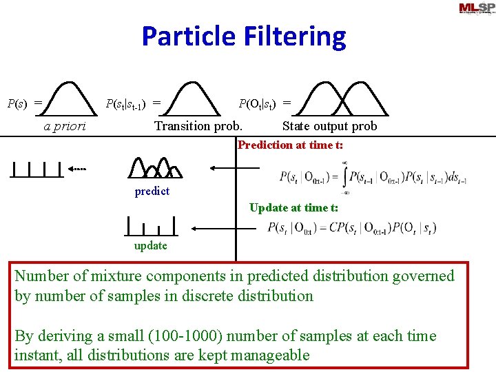
Particle Filtering P(st|st-1) = P(s) = a priori P(Ot|st) = Transition prob. State output prob Prediction at time t: sample predict Update at time t: update Number of mixture components in predicted distribution governed by number of samples in discrete distribution By deriving a small (100 -1000) number of samples at each time instant, all distributions are kept manageable

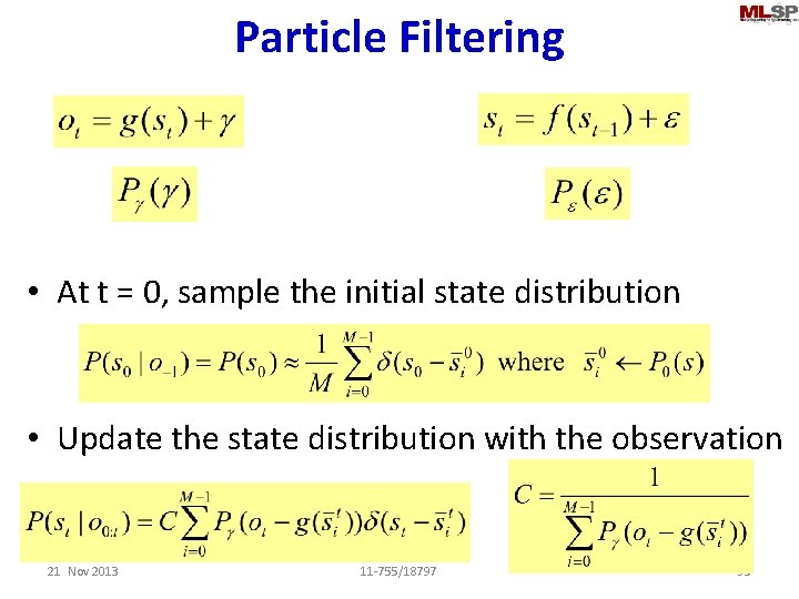
Particle Filtering • At t = 0, sample the initial state distribution • Update the state distribution with the observation 21 Nov 2013 11 -755/18797 95

Particle Filtering • Predict the state distribution at the next time • Sample the predicted state distribution 21 Nov 2013 11 -755/18797 96

Particle Filtering • Predict the state distribution at t • Sample the predicted state distribution at t • Update the state distribution at t 21 Nov 2013 11 -755/18797 97

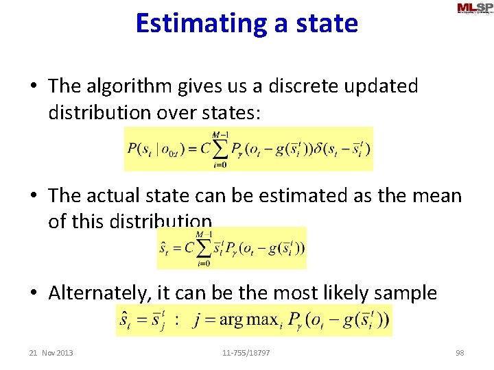
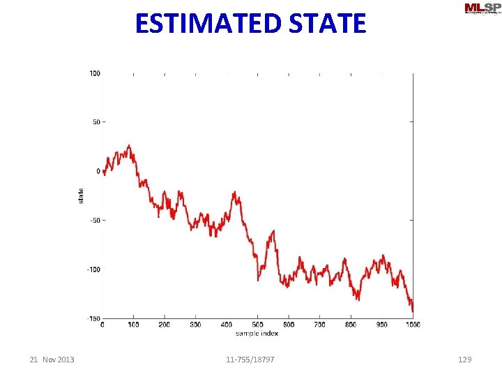
Estimating a state • The algorithm gives us a discrete updated distribution over states: • The actual state can be estimated as the mean of this distribution • Alternately, it can be the most likely sample 21 Nov 2013 11 -755/18797 98

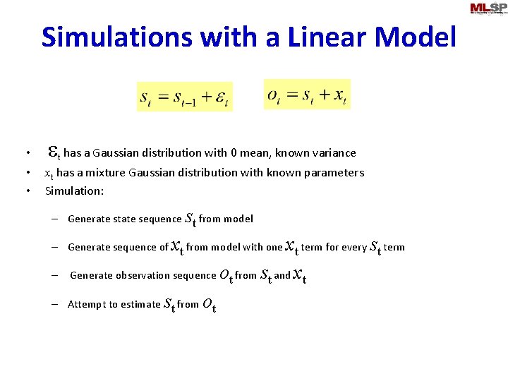
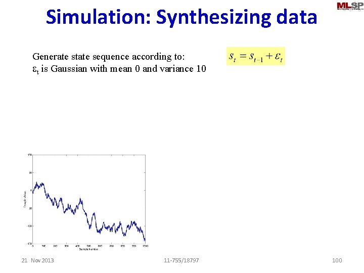
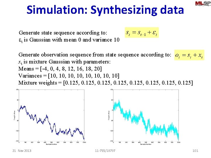
Simulations with a Linear Model • e has a Gaussian distribution with 0 mean, known variance • • xt has a mixture Gaussian distribution with known parameters Simulation: t s – Generate state sequence t from model x x Generate observation sequence ot from st and xt Attempt to estimate st from ot s – Generate sequence of t from model with one t term for every t term – –

Simulation: Synthesizing data Generate state sequence according to: et is Gaussian with mean 0 and variance 10 21 Nov 2013 11 -755/18797 100

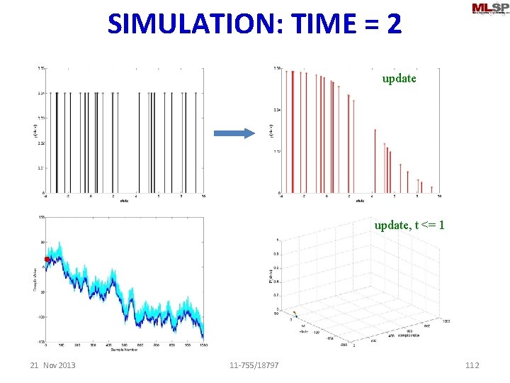
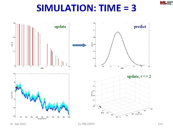
Simulation: Synthesizing data Generate state sequence according to: et is Gaussian with mean 0 and variance 10 Generate observation sequence from state sequence according to: xt is mixture Gaussian with parameters: Means = [-4, 0, 4, 8, 12, 16, 18, 20] Variances = [10, 10, 10] Mixture weights = [0. 125, 0. 125] 21 Nov 2013 11 -755/18797 101

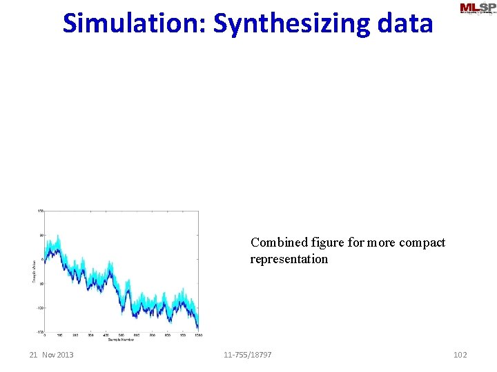
Simulation: Synthesizing data Combined figure for more compact representation 21 Nov 2013 11 -755/18797 102

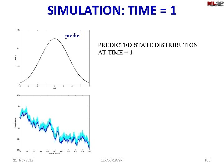
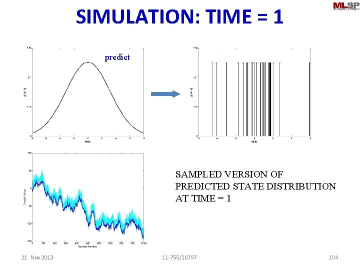
SIMULATION: TIME = 1 predict PREDICTED STATE DISTRIBUTION AT TIME = 1 21 Nov 2013 11 -755/18797 103

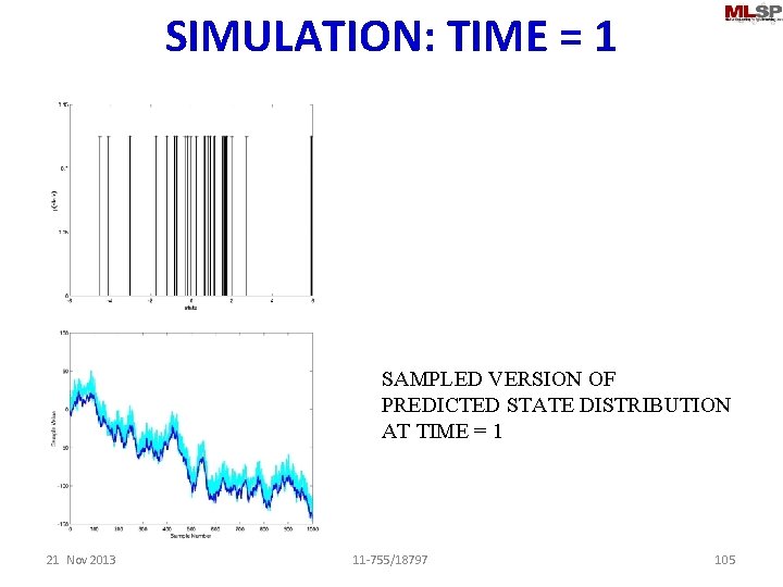
SIMULATION: TIME = 1 sample predict SAMPLED VERSION OF PREDICTED STATE DISTRIBUTION AT TIME = 1 21 Nov 2013 11 -755/18797 104

SIMULATION: TIME = 1 sample SAMPLED VERSION OF PREDICTED STATE DISTRIBUTION AT TIME = 1 21 Nov 2013 11 -755/18797 105

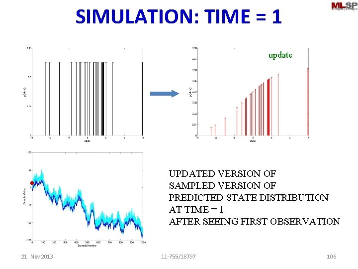
SIMULATION: TIME = 1 sample update UPDATED VERSION OF SAMPLED VERSION OF PREDICTED STATE DISTRIBUTION AT TIME = 1 AFTER SEEING FIRST OBSERVATION 21 Nov 2013 11 -755/18797 106

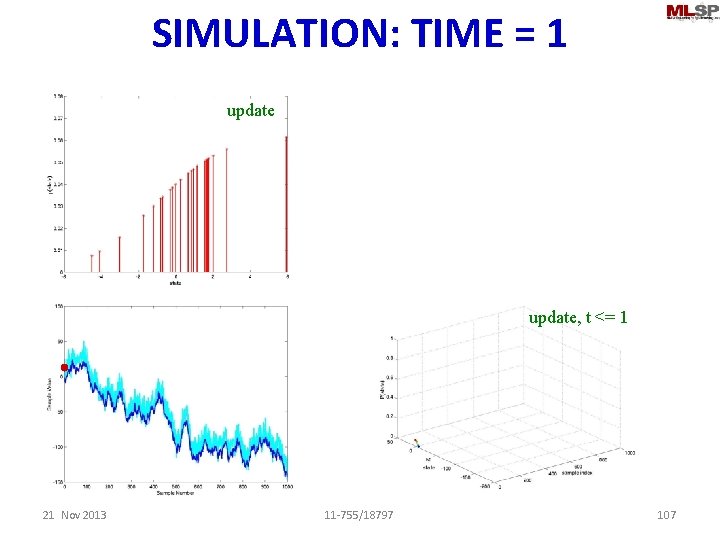
SIMULATION: TIME = 1 update, t <= 1 21 Nov 2013 11 -755/18797 107

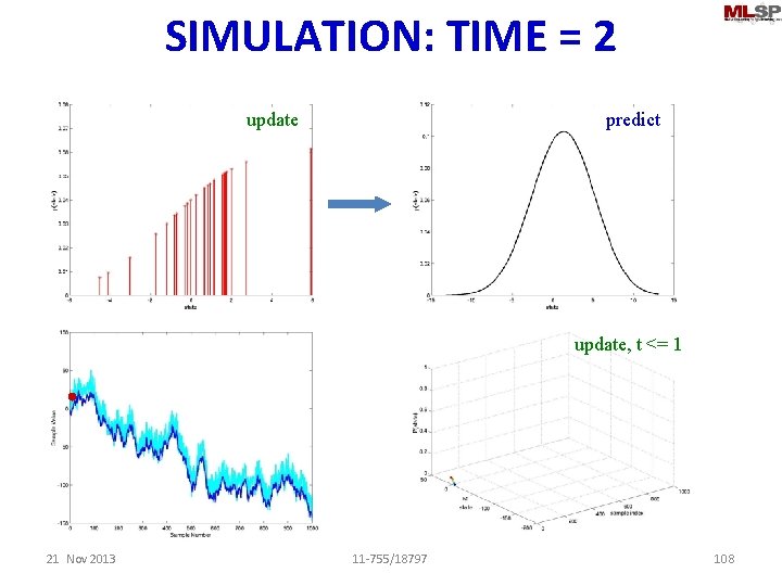
SIMULATION: TIME = 2 update predict update, t <= 1 21 Nov 2013 11 -755/18797 108

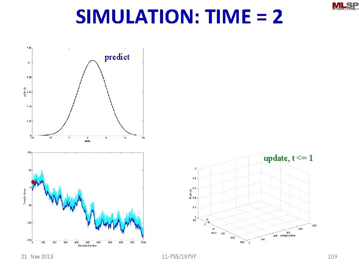
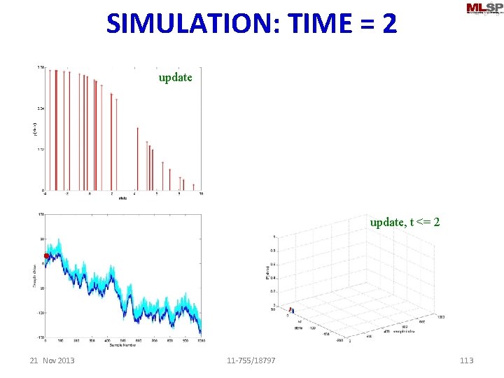
SIMULATION: TIME = 2 predict update, t <= 1 21 Nov 2013 11 -755/18797 109

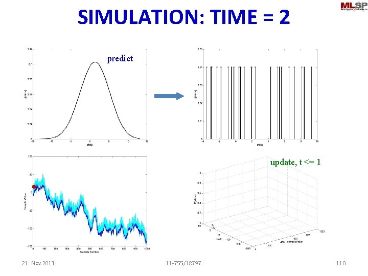
SIMULATION: TIME = 2 sample predict update, t <= 1 21 Nov 2013 11 -755/18797 110

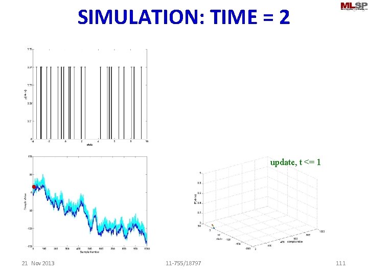
SIMULATION: TIME = 2 sample update, t <= 1 21 Nov 2013 11 -755/18797 111

SIMULATION: TIME = 2 sample update, t <= 1 21 Nov 2013 11 -755/18797 112

SIMULATION: TIME = 2 update, t <= 2 21 Nov 2013 11 -755/18797 113

SIMULATION: TIME = 3 update predict update, t <= 2 21 Nov 2013 11 -755/18797 114

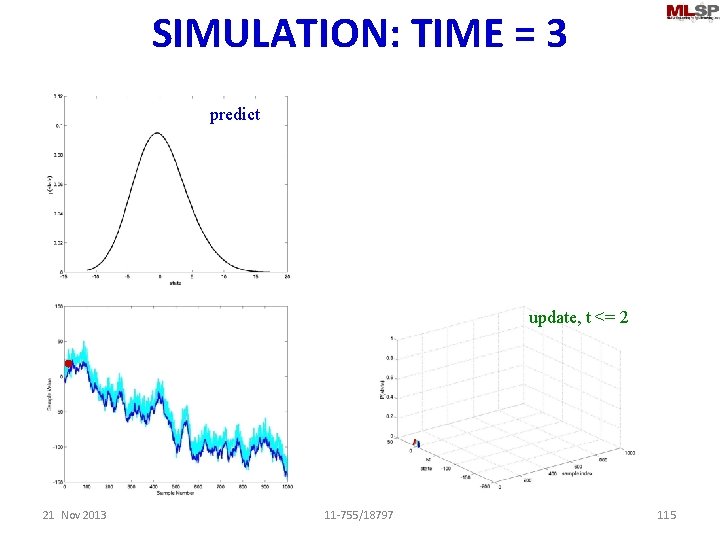
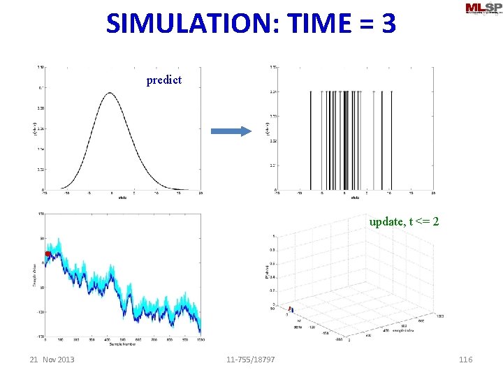
SIMULATION: TIME = 3 predict update, t <= 2 21 Nov 2013 11 -755/18797 115

SIMULATION: TIME = 3 sample predict update, t <= 2 21 Nov 2013 11 -755/18797 116

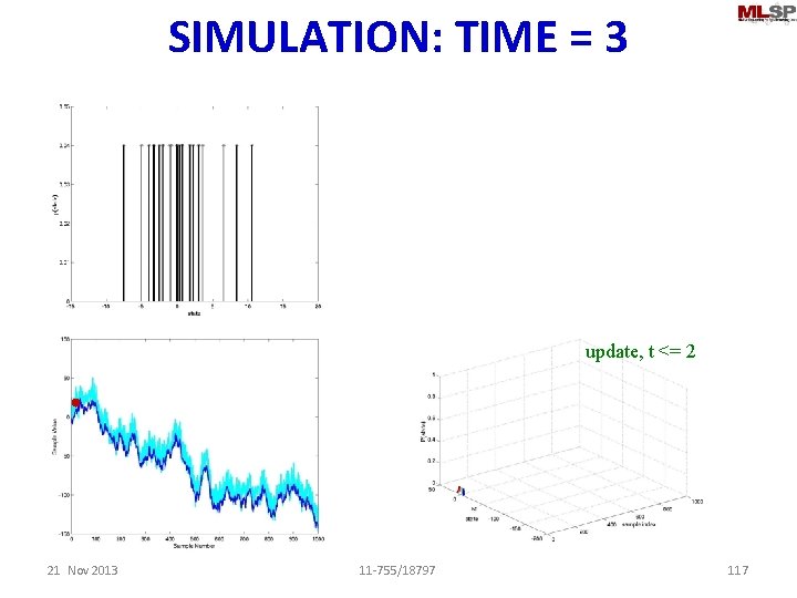
SIMULATION: TIME = 3 sample update, t <= 2 21 Nov 2013 11 -755/18797 117

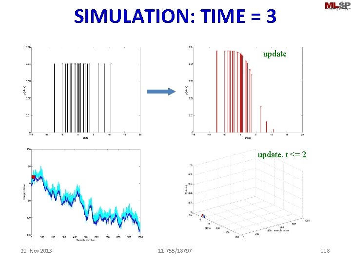
SIMULATION: TIME = 3 sample update, t <= 2 21 Nov 2013 11 -755/18797 118

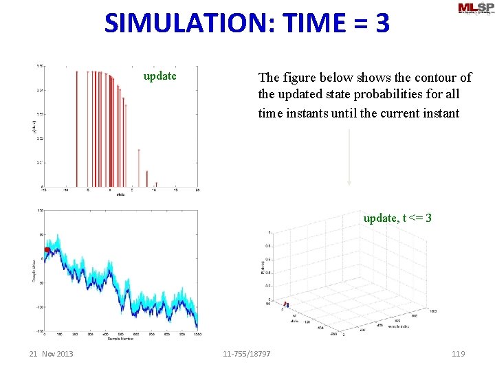
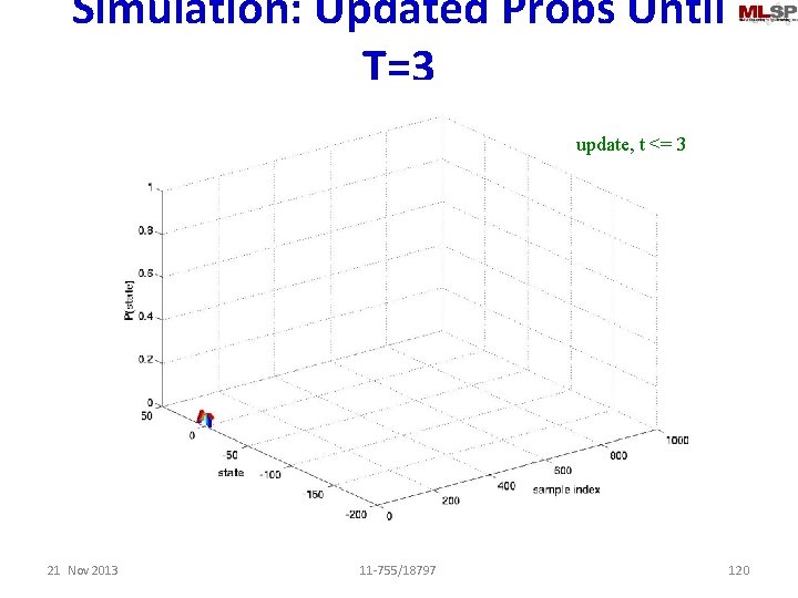
SIMULATION: TIME = 3 update The figure below shows the contour of the updated state probabilities for all time instants until the current instant update, t <= 3 21 Nov 2013 11 -755/18797 119

Simulation: Updated Probs Until T=3 update, t <= 3 21 Nov 2013 11 -755/18797 120

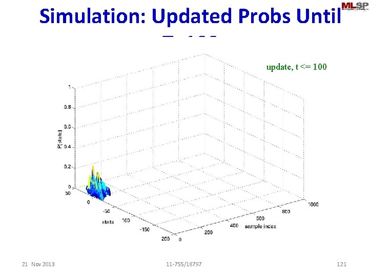
Simulation: Updated Probs Until T=100 update, t <= 100 21 Nov 2013 11 -755/18797 121

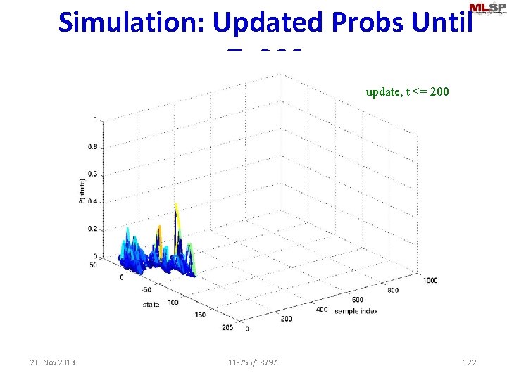
Simulation: Updated Probs Until T=200 update, t <= 200 21 Nov 2013 11 -755/18797 122

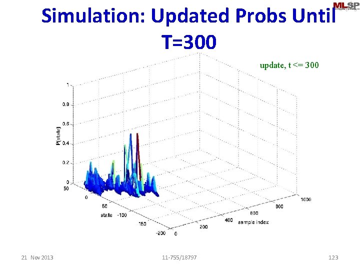
Simulation: Updated Probs Until T=300 update, t <= 300 21 Nov 2013 11 -755/18797 123

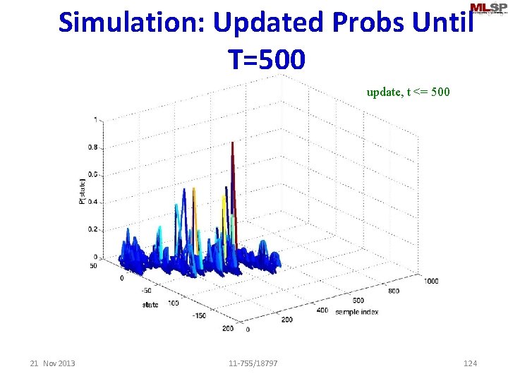
Simulation: Updated Probs Until T=500 update, t <= 500 21 Nov 2013 11 -755/18797 124

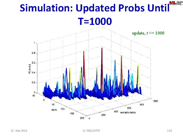
Simulation: Updated Probs Until T=1000 update, t <= 1000 21 Nov 2013 11 -755/18797 125

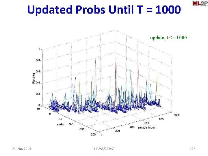
Updated Probs Until T = 1000 update, t <= 1000 21 Nov 2013 11 -755/18797 126

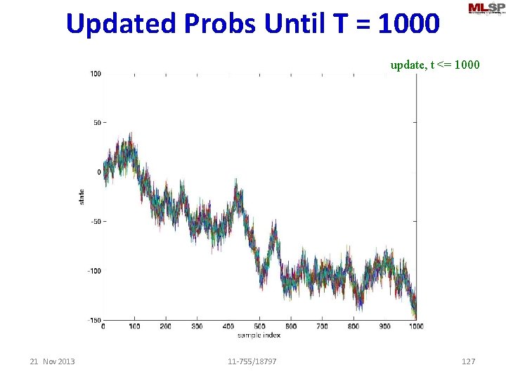
Updated Probs Until T = 1000 update, t <= 1000 21 Nov 2013 11 -755/18797 127

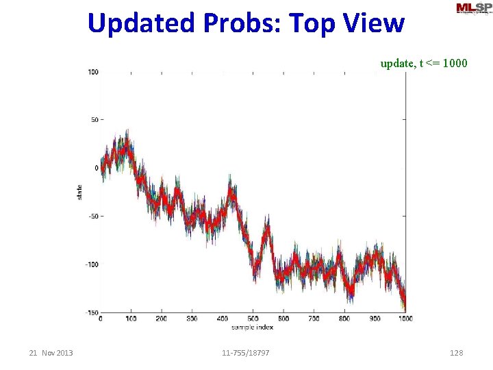
Updated Probs: Top View update, t <= 1000 21 Nov 2013 11 -755/18797 128

ESTIMATED STATE 21 Nov 2013 11 -755/18797 129

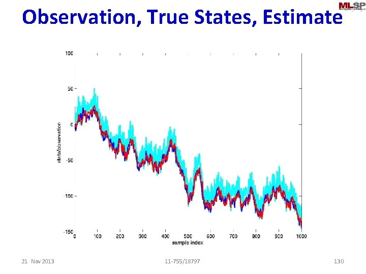
Observation, True States, Estimate 21 Nov 2013 11 -755/18797 130

Particle Filtering • Generally quite effective in scenarios where EKF/UKF may not be applicable – Potential applications include tracking and edge detection in images! – Not very commonly used however • Highly dependent on sampling – A large number of samples required for accurate representation – Samples may not represent mode of distribution – Some distributions are not amenable to sampling • Use importance sampling instead: Sample a Gaussian and assign nonuniform weights to samples 21 Nov 2013 11 -755/18797 131

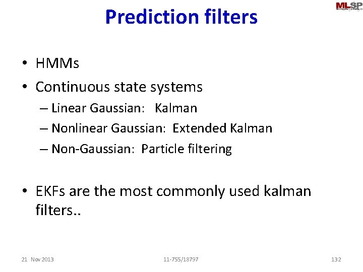
Prediction filters • HMMs • Continuous state systems – Linear Gaussian: Kalman – Nonlinear Gaussian: Extended Kalman – Non-Gaussian: Particle filtering • EKFs are the most commonly used kalman filters. . 21 Nov 2013 11 -755/18797 132