Geotechnical Engineering II CE 481 Shear Strength of

Geotechnical Engineering II CE 481 Shear Strength of Soil Chapter 10: Sections# 10. 2 and 10. 3 Chapter 12: All sections except 12. 13, 12. 14, 12. 15, 12. 17, 12. 18

Topics q Introduction q Basic Principles q Components of Shear Strength of Soils q Normal and Shear Stresses on a Plane q Mohr-Coulomb Failure Criterion q Laboratory Shear Strength Testing • • • Direct Shear Test Triaxial Compression Test Unconfined Compression Test q Field Testing (Vane test) q Stress Path

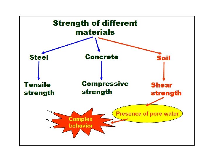
INTRODUCTION o Soil failure usually occurs in the form of “shearing” along internal surface within the soil. o The shear strength of a soil mass is the internal resistance per unit area that the soil mass can offer to resist failure and sliding along any plane inside it. o The safety of any geotechnical structure is dependent on the strength of the soil. o Shear strength determination is a very important aspect in geotechnical engineering. Understanding shear strength is the basis to analyze soil stability problems like: • Bearing capacity. • Lateral pressure on earth retaining structures • Slope stability

Bearing Capacity Failure Strip footing Failure surface Mobilized shear resistance At failure, shear stress along the failure surface (mobilized shear resistance) reaches the shear strength.

Bearing Capacity Failure Transcona Grain Elevator, Canada (Oct. 18, 1913)

Bearing Capacity Failure

Slope Failure At failure, shear stress along the failure surface ( ) reaches the shear strength ( f). The soil grains slide over each other along the failure surface.

Slope Failure

Failure of Retaining Walls Retaining wall Mobilized shear resistance Failure surface At failure, shear stress along the failure surface (mobilized shear resistance) reaches the shear strength.

Topics q Introduction q Basic Principles q Components of Shear Strength of Soils q Normal and Shear Stresses on a Plane q Mohr-Coulomb Failure Criterion q Laboratory Shear Strength Testing • • • Direct Shear Test Triaxial Compression Test Unconfined Compression Test q Field Testings (Vane test) q Stress Path

BASIC PRINCIPLES The brick (solid block) is in equilibrium under its own weight W and the opposite and equal reaction N. A horizontal force Sa is applied: i) If Sa is relatively small then the brick will remain at rest and Sa will be balanced by an equal and opposite force Sr. ii) As Sa increases, Sr will also increase with the same magnitude until Sa exceeds a certain limit, then the brick will move. This movement or slippage is a shear failure, where • Sa is applied shearing force • Sr is shearing resistance. Up to the moment of failure Sr = Sa. N R Sa Extra W W d N Question: What is the magnitude of Sa required to move the brick (i. e. to cause failure) Sr R/

Answer: That mainly depends on two factors: Extra 1. The friction between the brick and the table. The larger the value of (static) friction coefficient the larger is Sa required to move the brick. 2. The weight of the brick. The larger is W the larger is Sa necessary for sliding. In general Sa = W. tan …… (1) Sr = N. tan d ……. (2) is called the obliquity of the resultant or simply the obliquity angle. d is called the DEVELOPED FRICTION ANGLE Since N = W, and Sr = Sa then d = ………. . (3) Equation (3) is true up until the moment of sliding. When the applied shearing resistance Sa reaches a certain value Saf, which has an obliquity angle m, then

• The obliquity angle d reaches its maximum . • The shearing resistance Sr has reached its maximum possible value for the material. Ø is called the FRICTION ANGLE Ø Srf is called the SHEAR STRENGTH R W m From Eq. (2) Srf = N. tan ………(4) Or if we use only one subscript for clarity Saf N Sf = N. tan …. …. (5) If we divide by the cross-sectional area f = n. tan … …. (6) In which f = the shearing strength (shearing stress at failure) n = Normal stress acting on the failure plane = Friction angle Extra Sr f R/

Topics q Introduction q Basic Principles q Components of Shear Strength of Soils q Normal and Shear Stresses on a Plane q Mohr-Coulomb Failure Criterion q Laboratory Shear Strength Testing • • • Direct Shear Test Triaxial Compression Test Unconfined Compression Test q Field Testing (Vane test) q Stress Path

SHEAR STRENGTH OF SOILS o Coulomb (1776) observed that there was a stress-dependent component of shear strength and a stress-independent component. o The stress-dependent component is similar to sliding friction in solids described above. The other component is related to the intrinsic COHESION of the material. Coulomb proposed the following equation for shear strength of soil: cohesion Friction f = shear strength of soil n = Applied normal stress C = Cohesion = Angle of internal friction (or angle of shearing resistance)

o Cohesion (c), is a measure of the forces that cement particles of soils (stress independent). o Internal Friction angle (φ), is a measure of the shear strength of soils due to friction (stress dependent). o For granular materials, there is no cohesion between particles and Eq. (7) is reduced to

o We can see that Eq. 6 and Eq. 8 are identical. o Physically is it the case? Answer: o Although the two equations are the same, however, the difference is in the meaning of . • In solids is dependent on the roughness or friction of the sliding solids. • In granular soils, the friction angle represents the sum of sliding friction and interlocking. Therefore, it is designated angle of internal friction. o Where is sliding friction is more or less constant in a given soil, interlocking is dependent on 1. Particle shape and size 2. Densification o But both sliding and lifting depend on the applied normal stress.

o For cohesive soils cohesion is not equal to zero and Eq. 7 holds true. Cohesion is high especially for overconsolidated clays. Important notes: . o Even though in clay the relation between f and n is related to the angle , however in clay the nature of is not the same as the friction angle of granular soil or of solids in contact. o Soil derives its shear strength from two sources: • Cohesion: between particles - Cementation between sand grains - Electrostatic attraction between clay particles • Frictional resistance: between particles

Saturated Soils But from the principle of effective stress Where u is the pore water pressure (p. w. p. ) Then Eq. (9) becomes o C , or C’ , ’ are called strength parameters, and we will discuss various laboratory tests for their determination. o But before that we need to know what is failure. This, on the other hand, requires specification of the failure plane in order to find n in Eq. 11.

Topics q Introduction q Basic Principles q Components of Shear Strength of Soils q Normal and Shear Stresses on a Plane q Mohr-Coulomb Failure Criterion q Laboratory Shear Strength Testing • • • Direct Shear Test Triaxial Compression Test Unconfined Compression Test q Field Testing (Vane test) q Stress Path

Review of Basic Concepts I. Normal and Shear Stress along a Plane We will consider only two-dimensional case x y yx xy x xy Soil element yx y Since the soil element is in equilibrium, it follows by taking moments about any corner that xy = yx o Note that for convenience our sign convention has compressive forces and stresses positive because most normal stresses in geotechnical engineering are compressive. o These conventions are the opposite of those normally assumed in structural mechanics.

• We want to find normal stress n and shear stress n on plane EF which makes an angle with x-direction y N xy D x n C xy n F x A x xy xy B y T E xy xy B y • To obtain n and n, we sum the components of forces that act on the element in the N and T directions. • Assume the area of EF = 1 Then the area of EB = 1. cos The area of FB = 1. Sin y > x

For Normal stress along plane ( n): N n n F x xy T . . . (1) E xy B y For Shear stress along plane ( n): Equation (1) and (2) can be used to calculate NORMAL and shearing stresses on any plane making an angle with the x-direction. . . (2)

II. Principal Planes and Principal Stresses o From Eq. (2) we can see that at a certain angle , the shear stress will be equal to zero p . . . (3) o For given values of xy , x , y Eq (3) will give two values of p which are 90 o apart. This means that there are two PLANES that are at right angles to each other on which the shear stress is zero. o Such planes are called PRINCIPAL PLANES and the normal stress acting on them are termed PRINCIPAL STRESSES. o These principle stresses are obtained by substituting Eq. (3) into Eq. (1) to get:

Major Principal Stress: . . (4) Minor Principal Stress: . . . . (5) Now in terms of principal stress Eq. (1) and Eq. (2) becomes . . . . (6) . . . (7) Note: Eqs. (4) and (5) can also be obtained by differentiating Eq. (1) with respect to 2 to get the maximum and minimum values of n. Therefore we can conclude that: • For planes with major and minor principal stresses the value of shear stress is zero.

II. Maximum shear stress The maximum shear stress can be obtained by differentiating Eq. (2) w. r. t 2 , i. e. Eq. (8) is the negative reciprocal of Eq. (3). ……. (9) ……. (10) It is clear from Eqs. (4), (5) and (10) that. ………. . (11) Note We could simply reach Eq. 11 from Eq. 7. Check that Dealing with principal planes is easier as only we have two terms instead of three.

In brief Now from Eqs. 1 through 11 we could find: • The analytical procedure is sometimes awkward to use in practice. • We will discuss now a graphical procedures which will enable us to find the above without the hassle of going over many equations.

III. Graphical Method Representation of State of Stress Extra In terms of principal stress, normal and shear stress on a plane inclined at an angle are given by Eq. 6 and Eq. 7, respectively. From Eq. (7) . . …. (12) From the figure across 2 . . …. (13) Substituting Eq. (13) into Eq. 6 yields ……. . (14) Squaring Eq. (14) gives

Notes o When the circle of Eq. (15) is plotted in - space, it is known as the Mohr’s Circle of stress (Mohr, 1887). It represents the state of stress at a POINT at EQUILIBRIUM and it applies to any material, not just a soil. o Mohr’s Circle is a two-dimensional graphical representation of the state of stress at a point. o The scales of and have to be the same to obtain a circle from Eq. (15). o The Mohr’s circle construction enables the stresses acting in different directions at a point on a plane to be determined, provided that the stress acting normal to the plane is a principal stress. o The normal stress and shear stress that act on any plane can also be determined by plotting a Mohr’s circle.

Sign Convention in Mohr’s circle Shear stress, ( x, xy) y Normal stress, x xy ( y, - xy) x y Sign Convention yx Normal Stresses yx xy Shear Stresses Positive Compression Counter clockwise rotation Negative Tension Clockwise rotation

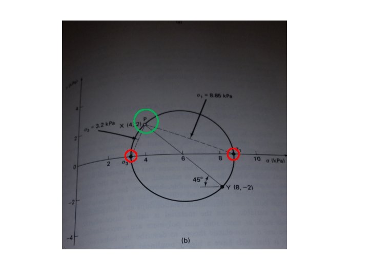
• Construction of Mohr’s Circle 1. Plot σy, xy as point M 2. Plot σx, xy as point R 3. Connect M and R 4. Draw a circle of diameter of the line RM about the point where the line RM crosses the horizontal axis (denote this as point O) Note: We could construct two additional Mohr circles for 1 and 2 and 3 to complete Mohr diagram. o The points R and M in Fig. (b) above represent the stress conditions on plane AD and AB, respectively. O is the point of intersection of the normal stress axis with the line RM.

o The circle MNQRS drawn with O as the center and OR as the radius is Mohr’s circle for the stress conditions considered. The radius of the Mohr’s circle is equal to o The stress on plane EF can be determined by moving an angle 2 (which is twice the angle that the plane EF makes in a counterclockwise direction with plane AB) in a counterclockwise direction from point M along the circumference of the Mohr’s circle to reach point Q. The abscissa and ordinate of point Q, respectively, give the normal stress n and the shear stress n on plane EF. o Because the ordinates (that is, the shear stresses) of points N and S are zero, they represent the stresses on the principal planes. The abscissa of point N is equal to 1 and the abscissa for point S is 3.

Special Case Next we will see a more powerful method for finding stress on any plane.

Pole Method for Finding Stresses on a Plane o There is a unique point on the Mohr’s circle called the POLE or the ORIGIN of PLANES. This point has a very useful property: Any straight line drawn through the pole will intersect the Mohr’s circle at a point which represents the state of stress on a plane inclined at the same orientation in space as the line. o This concept means that if you know the state of stress, and , on some plane in space, you can draw a line parallel to that plane through the coordinates of and on the Mohr circle. o The pole then is the point where that line intersects the Mohr circle. o Once the pole is known, the stresses on any plane can readily be found by simply drawing a line from the pole parallel to that plane; the coordinates of the point of intersection with the Mohr circle determine the stresses on that plane.

How to determine the location of the Pole? Shear stress, yx ( n, n) on plane EF ( x, xy) x y F xy E x y 2 P yx xy Normal stress, ( y, - xy) Note: it is assumed that y > x 1. From a point of known stress coordinates and plane orientation, draw a line parallel to the plane where the stress is acting on. 2. The line intersecting the Mohr circle is the pole, P.

Shear stress, Using the Pole to Determine Principal Planes yx y 1 ( x, xy) x xy x E y 3 Normal stress, p P Direction of Minor Principal Plane ( y, - xy) F Direction of Major Principal Plane yx xy

Example 1 For the stresses of the element shown across, determine the normal stress and the shear stress on the plane inclined at = 35 o from the horizontal reference plane. Solution § Plot the Mohr circle to some convenient scale (See the figure across). § Establish the POLE § Draw a line through the POLE inclined at angle = 35 o from the horizontal plane it intersects the Mohr circle at point C. = 39 k. Pa = 18. 6 k. Pa You should verify these results by using Eqs. (6), (7)

Example 2 The same element and stresses as in Example 1 except that the element is rotated 20 o from the horizontal as shown. Solution § Since the principal stresses are the same, the Mohr circle will be the same as in Example 1. § Establish the POLE. § Draw a line through the POLE inclined at angle = 35 o from the plane of major principal stress. It intersects the Mohr circle at point C. § The coordinates of point C yields = 39 k. Pa = 18. 6 k. Pa

REMARKS § and are the same as in example 1. Why is this? Because nothing has changed except the orientation in space of the element. § We could just as well have used the minor principal plane as our starting point to establish the POLE. § We could just as well rotate the - axis to coincide with the directions of the principal stresses in space, but traditionally versus is plotted with the axes horizontal and vertical. § We can see that the Mohr circle of stress represents the complete two-dimensional state of stress at equilibrium in an element or at a point. § The pole simply couples the Mohr circle to the orientation of the element in the real world. § The Mohr circle and the concept of the POLE are very useful in geotechnical engineering. § The construction of Mohr’s circle is one of the few graphical techniques still used in engineering. It provides a simple and clear picture of an otherwise complicated analysis.

Example 3

Example 4 y 8 k 4 k N N/ m 2 8 k N/ x N/ m 2 y 4 k 45 o m 2 2 k N/ m 2 x /m 2 Given the stress shown on the element across. Find the magnitude and direction of the major and minor principal stresses.

Topics q Introduction q Basic Principles q Components of Shear Strength of Soils q Normal and Shear Stresses on a Plane q Mohr-Coulomb Failure Criterion q Laboratory Shear Strength Testing • • • Direct Shear Test Triaxial Compression Test Unconfined Compression Test q Field Testing (Vane test) q Stress Path

FAILURE CRITERIA FOR SOILS o There are many ways of defining failure in real materials, or put another way, there are many failure criteria. o Various theories are available for different engineering materials. However, no one is general for all materials o The one generally accepted and used for soil is Mohr Theory of Failure. o According to Coulomb relation for shear strength What is the failure plane? • Is it the plane with the maximum shear stress? …. No. • Is it the plane of the maximum normal stress (i. e. major principal stress)…. No.

Mohr Theory of Failure Mohr theory of failure states that: A material fails along the plane and at the time at which the angle between the RESULTANT of the NORMAL and SHEARING STRESS and the NORMAL STRESS is a maximum; that is , when the combination of NORMAL and SHEARING stresses produces the maximum obliquity angle m. n 1 D 3 2 f O m qf A Pole 3 1 C n 2 B

o In the across diagram, it is seen that the optimum stress combination which fulfills Mohr’s criterion is that represented by the point D, and the orientation of the failure plane is represented by the line AD which makes an angle f with the maximum principal plane. n D 2 f O m qf C n 2 B A Pole 3 1 o Since, according to the Mohr theory, the tangent line OD represents the stress situation at failure, the maximum obliquity angle m is equal to the friction angle , just as indicated in the case of the brick sliding on a horizontal surface.

Mohr Failure Envelope o By plotting Mohr’s circles for different states of stresses and in each case draw a tangent to each circle from the origin we come up with points 1, 2, 3… etc. If we connect those points we come up with what is called Mohr’s failure envelope. • C 2 • B Mohr failure envelope • A 1 3 c 3 3 b 1 c 3 a 1 b 1 a

o This envelope separates cases of stresses which cause failure from that which do not. o For instance if the normal stress and shear stress on a plane in a soil mass are such that they plot as point A shown above, shear failure will not occur along that plane. o For point B failure takes place, and point C cannot exist, since it plots above failure envelope and shear failure in a soil would have occurred already. o Therefore, failure occurs only when the combination of shear and normal stress is such that the Mohr circle is TANGENT to the Mohr failure envelope.

Mohr-Coulomb Failure Criterion o The disadvantages of Mohr failure envelope is that it is a curved line, and needs a lot of tests to construct and difficult to use. o It was then approximated to be a straight line, and the equation for the line was written in terms of the Coulomb strength parameters C and , as o This gave the birth to MOHR-COULOMB FAILURE CRITERION, which is by far the most popular criterion applied to soils. f c tan c ’f coh ent n o mp o c e esiv ' frictional component

Orientation of Failure Plane 1 3 h f 90+ Pole Once we assume straight line failure envelope, qf = 45 + /2 always and independent of the values of s 1 and s 3 (i. e. confinement). v + 2 qf = 90 + f qf = 45 + f/2 This could be proved analytically (See Das)

Mohr circles & failure envelope in terms of total and effective stress

Mohr-Coulomb Failure Criterion in terms of effective stress u = pore water pressure pe o l e env re u l i fa Effective cohesion f c’ ’f ’ C’ and ’ are called the effective strength parameters. Effective friction angle ’ In this case, soil behavior is controlled by effective stresses, and the effective strength parameters are the fundamental strength parameters.

Mohr-Coulomb Failure Criterion in terms of total stress e f Cohesion re ailu f c f lop e v n e Friction angle f is the maximum shear stress the soil can take without failure, under normal stress of .

What does the Failure Envelope Signify? (will not exist) ( failure) (no failure) q If the magnitudes of and on plane ab are such that they plot as point A shear failure will not occur along the plane. q If the effective normal stress and the shear stress on plane ab plot as point B (which falls on the failure envelope), shear failure will occur along that plane. q A state of stress on a plane represented by point C cannot exist, because it plots above the failure envelope, and shear failure in a soil would have occurred already.

Mohr Circles & Failure Envelope Failure surface X Y ’ Soil elements at different locations Y ~ stable X ~ failure

Mohr Circles & Failure Envelope The soil element does not fail if the Mohr circle is contained within the envelope GL v Y h h v v+

Mohr Circles & Failure Envelope As loading progresses, Mohr circle becomes larger… GL Failure point v Y h h. . and finally failure occurs when Mohr circle touches the envelope

Relationship between principle stresses and shear strength parameters

Relationship between principle stresses and shear strength parameters

Remarks o C and are measures of shear strength and are called shear strength parameters. o The parameters C, are in general not soil constants. They depend on the initial state of the soil (e. g. density, water content), and type of loading (drained or undrained). o In case of using effective stress, C’ and ’ are called effective shear strength parameters. o The value of C’ for sand inorganic silt is 0. For normally consolidated clays, C’ can be approximated at 0. Overconsolidated clays have values of C’ that are greater than 0.

Topics q Introduction q Basic Principles q Components of Shear Strength of Soils q Normal and Shear Stresses on a Plane q Mohr-Coulomb Failure Criterion q Laboratory Shear Strength Testing • • • Direct Shear Test Triaxial Compression Test Unconfined Compression Test q Field Testing (Vane test) q Stress Path

Laboratory Shear Strength Testing o The purpose of laboratory testing is to determine the shear strength parameters of soil (C, or C’, ’) through the determination of failure envelope. o The shear strength parameters for a particular soil can be determined by means of laboratory tests on specimens taken from representative samples of the in-situ soil. o There are several laboratory methods available to determine the shear strength parameters (i. e. C, , C’, ’). Some of the tests are rather complicated. o For further details you should consult manuals and books on laboratory testing, especially those by the ASTM.

Determination of shear strength parameters of soils (C, or C’, ’) Laboratory Tests Most common laboratory tests to determine the shear strength parameters are, 1. Direct shear test 2. Triaxial shear test Other laboratory tests include: • Direct simple shear test • Torsional or ring shear test • Hollow cylinder test • Plane strain triaxial test • Laboratory vane shear test • Laboratory fall cone test. Field Tests 1. Standard penetration test Pressuremeter 2. Vane shear test 3. Pocket penetrometer 4. Static cone penetrometer Field test equipment and test methods are described in most textbooks on foundation engineering.

Laboratory testing must simulate field conditions and loading Failure surface Y Triaxial Shear test X Direct Shear test Soil elements at different locations

vc + Laboratory tests Simulating field conditions in the laboratory 0 vc hc vc + vc ct sh vc 0 Representative soil sample taken from the site i Tr Di re 0 hc 0 l ia x a hc st e t ea rt es t vc Step 1 Set the specimen in the apparatus and apply the initial stress condition Step 2 Apply the corresponding field stress conditions

• In laboratory, a soil sample can fail in two ways: Way 1: Increase normal stress ( 1) to failure with confining stress ( 3) constant Way 2: Normal stress is applied and held constant then shear stress is applied to failure Normal Stress, n 1 Shear Stress, 3 3 1 Triaxial Shear Test n Direct Shear Test

Topics q Introduction q Basic Principles q Components of Shear Strength of Soils q Normal and Shear Stresses on a Plane q Mohr-Coulomb Failure Criterion q Laboratory Shear Strength Testing • • • Direct Shear Test Triaxial Compression Test Unconfined Compression Test q Field Testing (Vane test) q Stress Path

Determination of shear strength parameters of soils (C, or C’, ’) Laboratory Tests Most common laboratory tests to determine the shear strength parameters are, 1. Direct shear test 2. Triaxial shear test Other laboratory tests include: • Direct simple shear test • Torsional or ring shear test • Hollow cylinder test • Plane strain triaxial test • Laboratory vane shear test • Laboratory fall cone test. Field Tests 1. Standard penetration test Pressuremeter 2. Vane shear test 3. Pocket penetrometer 4. Static cone penetrometer Field test equipment and test methods are described in most textbooks on foundation engineering.

Direct Shear Test P Steel ball Pressure plate Porous plates S Soil Proving ring to measure shear force

Preparation of a sand specimen Porous plates Components of the shear box Preparation of a sand specimen

Preparation of a sand specimen Pressure plate Leveling the top surface of specimen Specimen preparation completed

Test Procedure • A constant vertical force (normal stress) is applied through a metal platen. • Shear force is applied by moving one half of the box relative to the other and increased to cause failure in the soil sample. • The tests are repeated on similar specimens at various normal stresses • The normal stresses and the corresponding values of f obtained from a number of tests are plotted on a graph from which the shear strength parameters are determined.

Direct shear test Shear box Dial gauge to measure vertical displacement Proving ring to measure shear force Loading frame to apply vertical load Dial gauge to measure horizontal displacement

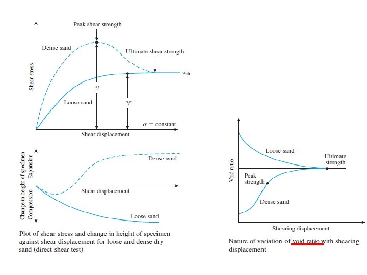
• The advantage of the strain-controlled tests is that in the case of dense sand, peak shear resistance (that is, at failure) as well as lesser shear resistance (that is, at a point after failure called ultimate strength) can be observed and plotted. • Compared with strain-controlled tests, stress-controlled tests probably model real field situations better.

Test results Normal Load : _____ kg Area of Sample: _____ cm 2 Horizontal Dial Reading (mm) Vertical Dial Reading (mm) Horizontal Shear Force (N) Shear Stress (k. Pa)

S h e a r s tr e s s , Stress-strain relationship Peak shear strength Dense sand/ OC clay Ultimate shear strength f f Loose sand/ NC clay Expansion Compression Change in height of the sample S h ear d i sp l acemen t Dense sand/OC Clay Shear displacement Loose sand/NC Clay

Determining strength parameters C and S h e a r s tr e s s , An example of testing three samples of a sand at the same relative density just before shearing. Normal stress = 3 Normal stress = 2 S h e a r s tr e s s a t fa i l u r e , f f 3 f 2 f 1 Normal stress = 1 S h ear d i sp l acemen t Mohr – Coulomb failure envelope • Sand is cohesionless, then C = 0 • Direct shear tests are drained and pore water pressures are dissipated, then u = 0 • Therefore, = ’ N o r m a l s tr e s s , It is important to note that in situ cemented sands may show a C’ intercept.

In case of clay, horizontal displacement should be applied at a very slow rate to allow dissipation of pore water pressure (therefore, one test would take several days to finish) S h e a r s tr e s s a t fa i l u r e , f Failure envelopes for clay from drained direct shear tests Overconsolidated clay (C’ ≠ 0) Normally consolidated clay (c’ = 0) ’ N o r m a l s tr e s s ,

Notes on Direct Shear Test • This test is probably the oldest strength test because Coulomb used a type of shear box test more than two centuries ago to determine the necessary parameters for his strength equation. • The test is quick and inexpansive and common in practice. • Used to determine the shear strength of both cohesive as well as non-cohesive soils. • The test equipment consists of a metal box in which the soil specimen is placed. The box is split horizontally into two halves. • The shear test can be either stress controlled or strain controlled. • Tests on sands and gravels are usually performed dry. Water does not significantly affect the (drained) strength.

o Usually only relatively slow drained tests are performed in shear box apparatus. For clays rate of shearing must be chosen to prevent excess pore pressures building up. For sands and gravels tests can be performed quickly. o If there are no excess pore pressures and as the pore pressure is approximately zero the total and effective stresses will be identical. o The failure stresses thus define an effective stress failure envelope from which the effective (drained) strength parameters C’, ’ can be determined. o Normally consolidated clays (OCR = 1) and loose sands do not show separate peak and ultimate failure loci, and for soils in these states C’ = 0. o Overconsolidated clays and dense sands have peak strengths with C’ > 0.

Advantages of direct shear test o Inexpensive, fast, and simple, especially for granular materials. o Easiness of sample preparation in case of sand. o Due to the smaller thickness of the sample, rapid drainage can be achieved o Large deformations can be achieved by reversing shear direction. This is useful for determining the residual strength of a soil. o Samples may be sheared along predetermined planes. This is useful when the shear strengths along fissures or an interface is required.

Disadvantages of direct shear test o Failure occurs along a predetermined failure plane which may not be the weakest plane. o Non-uniform of shear stresses along failure surface in the specimen. There are rather stress concentrations at the sample boundaries, which lead to highly nonuniform stress conditions within the test specimen itself. o There is no means of estimating pore pressures, so effective stresses cannot be determined and only the total normal stress can be determined. o It is very difficult if not impossible to control drainage, especially for fine-grained soils. Consequently, the test is not suitable for other than completely drained conditions.

Example 1 A direct shear test was performed on a clay sample. The cross section are of the device is 6 cm x 6 cm. Normal Load (kg) Shear Load (kg) 360 260 720 380 1080 520 1440 640 Determine the shear envelope and shear strength parameters for the clay. Normal Load Normal Stress Shear Load at Shear Stress (kg) (kg/cm 2) failure at failure (kg) (kg/cm 2) 360 10 260 7. 22 720 20 380 10. 56 1080 30 520 14. 44 1440 40 640 17. 78

Normal Load Normal Stress Shear Load at Shear Stress (kg) (kg/cm 2) failure at failure (kg) (kg/cm 2) 360 10 260 7. 22 720 20 380 10. 56 1080 30 520 14. 44 1440 40 640 17. 78

Example 2 (Prob. # 3 in the text book) For a dry sand specimen in a direct shear test box, the following are given: • Size of specimen: 63. 5 mm 31. 75 mm (height) • Angle of friction: 33° • Normal stress: 193 k. N/m 2. Determine the shear force required to cause failure. = 193 tan (33) = 125. 33 k. Pa Shear force = 125. 33 x 0. 0635 = 0. 50538 k. N = 505. 38 N

Topics q Introduction q Basic Principles q Components of Shear Strength of Soils q Normal and Shear Stresses on a Plane q Mohr-Coulomb Failure Criterion q Laboratory Shear Strength Testing • • • Direct Shear Test Triaxial Compression Test Unconfined Compression Test q Field Testing (Vane test) q Stress Path

Triaxial Shear Test o The most reliable method now available for determination of shear strength parameters. o Entire books have been written on triaxial test. o The test is used to measure the shear strength of a soil under controlled drainage conditions. o The test is designed to simulate actual field conditions. representative soil sample z vc hc vc Before construction vc + hc z hc vc + After and during construction

o The test is called “triaxial” because three principle stresses are assumed to be known and controlled. o The triaxial test is much more complicated than the direct shear but also much more versatile. o The failure plane can occur anywhere and we can control the stress paths to failure reasonably well, which means that complex stress paths in the field can more effectively be modeled in the laboratory with the triaxial test.

Principles of Triaxial Test To simulate field conditions, soil samples is subjected to the following stages: 1. Saturation of sample (Check of B value) 2. Applying confining (cell) pressure ( 3) is applied on the soil sample. The confining pressure is within the range of that subjected in the field. 3. Apply an increasing vertical stress ( = 1 - 3) -termed the deviator stress- until failure. 4. The specimen is free to fail on any weak plane or, as sometimes occurs, to simply BULGE. Deviator Principle 3 Stress, or d 3 = Confining pressure = Cell pressure = All-around pressure 3 3 = 1 - 3

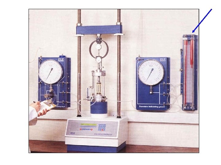
Triaxial Shear Test Device Two ways for appying axial load 1. Application of dead weights or hydraulic pressure in equal increments until the specimen fails. 2. Application of axial deformation at a constant rate by means of a geared or hydraulic loading press. This is a strain-controlled test.

Triaxial Shear Test Piston (to apply deviatoric stress) Failure plane O-ring Soil sample at failure Soil sample Perspex cell impervious membrane Porous stone Water Cell pressure Back pressure pedestal Pore pressure or volume change

Specimen preparation (undisturbed sample) Edges of the sample are carefully trimmed Setting up the sample in the triaxial cell

Apparatus Assembly Sample is covered with a rubber membrane and sealed Cell is completely filled with water

Apparatus Assembly Proving ring to measure the deviator load Dial gauge to measure vertical displacement

Types of Triaxial Tests o Many variations of test procedure are possible with the triaxial apparatus but the three principal types of test are as follows: Confining Pressure Shearing • Consolidated • Unconsolidated o Drained (CD) Test o Undrained (CU)Test o Undrained (UU) Test o Depends on whether drainage is allowed or not during the confining or shearing stage. o The different types of triaxial test are commonly designated by a two-letter symbol. The first letter refers to what happens BEFORE SHEAR that is whether the specimen is consolidated or not. The second letter refers to the drainage conditions during SHEAR, CD, CU, UU.

Types of Triaxial Tests deviator stress 3 Step 1 ( ) = 1 - 3 Step 2 3 3 3+ 3 Under Confining (cell) pressure 3 Is the drainage valve open? yes Consolidated sample no Unconsolidated sample Shearing (loading) Is the drainage valve open? yes no Drained Undrained loading

Types of Triaxial Tests Step 2 Step 1 Under Confining (cell) pressure 3 Is the drainage valve open? yes Consolidated sample no Shearing (loading) Is the drainage valve open? yes Unconsolidated sample Drained loading CD test UU test CU test no Undrained loading

Topics q Introduction q Basic Principles q Components of Shear Strength of Soils q Normal and Shear Stresses on a plane q Mohr-Coulomb Failure Criterion q Laboratory Shear Strength Testing • Direct Shear Test • Triaxial Compression Test (CD Test) • Unconfined Compression Test q Field Testing (Vane Test) q Stress Path

I. Consolidated Drained Test (CD Test) v No excess pore pressure throughout the test v Very slow shearing to avoid build-up of pore pressure hence this test is termed the S-test (for “slow” test) Can be days! v Gives C’ and ’ v Note that at all the times during CD test, the pore water pressure is essentially zero. Use C’ and ’ for analysing fully drained Situations (i. e. long term stability, very slow loading)

Piston (to apply deviatoric stress) O-ring Soil sample Perspex cell impervious membrane Porous stone Water Pore pressure or volume change Cell pressure Back pressure pedestal

Stress conditions for the consolidated drained test = Total, Neutral, u + Effective, ’ Step 1: At the end of consolidation 3 Drainage ’ 3 = 3 3 0 ’ 3 = 3 Step 2: During axial stress increase ’V = 3 + = ’ 1 3 + Drainage 3 0 ’h = 3 = ’ 3 Step 3: At failure ’Vf = 3 + f = ’ 1 f 3 + f Drainage 3 0 ’hf = 3 = ’ 3 f

In saturated soil, the change in the volume of the specimen ( Vc) that takes place during consolidation can be obtained from the volume of pore water drained. Volume change of specimen caused by chamber-confining pressure Volume change in loose sand normally consolidated clay during deviator stress application Volume change in dense sand overconsolidated clay during deviator stress application

Deviator stress, d Expansion Compression Volume change of the sample Stress-strain relationship during shearing Dense sand or OC clay ( d)f Loose sand or NC Clay Axial strain Dense sand or OC clay Axial strain Loose sand or NC clay

Deviator stress, d Strength parameters c’ and ’ Several tests on similar samples can be performed by varying the confining pressure. Then 3 and 1 at failure for each test are used to construct Mohr’s Circle. From that M-C failure envelope can be obtained. ( d)fc Confining stress = 3 b Confining stress = 3 a ( d)fb ( d)fa Shear stress, Axial strain Mohr – Coulomb failure envelope ve ti c e f Ef 3 a 1 = 3 + ( d)f ess r t s re u l i a e lop e e nv f = tan 3 ’ f 3 b 3 c 1 a ( d)fa 1 b ( d)fb 1 c ’

o The coordinates of the point of tangency of the failure envelope with Mohr’s circle give the stresses (normal and shear) on the failure plane of the respected test.

Failure envelopes for loose sand NC Clay o It is usually assumed that the C’ parameter for normally consolidated non-cemented clays is essentially zero for all practical purposes. Shear stress, o Therefore, one CD test would be sufficient to determine d of sand or NC clay ’ Mohr – Coulomb failure envelope 3 a 1 a ( d)fa ’

Failure envelopes for dense sand OC Clay NC OC c ’ b a c 3 ( d)f 1 c For portion ab of the failure envelope ’ For portion bc of the failure envelope

Can you think about Direct shear and Triaxial Test w. r. t. analysis of results n S h e a r s tr e s s , Normal stress = 3 that we plot Mohr circle and then we plot tangent to the circles (if is assumed = 0) only we need one circle) 1 = 3 + ( d)f 3 f 1 S h ear d i sp l acemen t Here we have n and for each test and we plot the M-C. If we need principal stress we plot Mohr circle which goes the point on the M-Cfor the concerned test f Mohr – Coulomb failure envelope Shear stress, f 2 Normal stress = 1 Deviator stress, d Normal stress = 2 f 3 S h e a r s tr e s s a t fa i l u r e , f 1 and 3 for each test from ( d)fc Confining stress = 3 b ( d)fa Confining stress = 3 a ’ 3 a 3 b 3 c 1 a Normal stress, ’ Axial strain 1 b 1 c

Example 1 For a normally consolidated clay specimen, the results of a drained triaxial test are as follows: • Chamber-confining pressure = 125 k. N/m 2 • Deviator stress at failure = 175 k. N/m 2 Determine the soil friction angle, ’ Solution 1 = 175+125 = 300 k. N/m 2 Sin ’ = ( 1 - 3)/( 1+ 3) ’ =24. 3 o Example 2 In a consolidated-drained triaxial test on a clay, the specimen failed at a deviator stress of 124 k. N/m 2. If the effective stress friction angle is known to be 31°, what was the effective confining pressure at failure? Solution We can solve it graphically. We know phi so we plot M-C envelope. ( 1 - 3)/2 equal the radius of Mohr circle Through trial we plot the circle that touch the M-C. From that we know 1 and 3 Sin 31 = ( 1 - 3)/( 1+ 3) = 124/Sin ( 1+ 3)=240 k. N/m 2 ( 1 - 3) =124 k. N/m 2 Two eqs. Two unknowns 1=182 k. N/m 2, 3= 58 k. N/m 2

Graphical Solution 200 150 31 o 100 50 100 If there is any slight difference from the analytical solution it is because the grid is not perfect square 150 200 250 300 Draw a circle with a radius of 62 and move it left until toughing the M-C envelope

Example 3 Samples of dry sand are to be tested in a direct shear and a triaxial test. In the triaxial test the sample fails when the major and minor principal stresses are 450 k. N/m 2 and 150 k. N/m 2, respectively. What shear strength be expected in the direct shear test when the normal loading is equal to a stress of 80 k. N/m 2. Solution Sin ’ = ( 1 - 3)/( 1+ 3) = (450 -150)/(450/150) = 0. 5 Hence ’ =30 o = n tan ’ = 80 tan 30 = 46. 2 k. N/m 2 Graphical Solution 200 150 30 o 100 50 100 150 200 250 300

Example 4 A conventional consolidated-drained (CD) triaxial test is conducted on a sand. The cell pressure is 100 k. N/m 2, and the applied axial stress at failure is 200 k. N/m 2. Required: a. Plot the Mohr circle for both the initial and failure stress conditions. b. The friction angle (Assume c = 0) c. The shear stress on the failure plane at failure. d. The theoretical angle of the failure plane in the specimen. e. The orientation of the plane of the maximum obliquity f. The maximum shear stress at failure and the angle of the plane on which it acts. g. The available shear strength on the plane of maximum shear and the factor of safety on this plane.

Required: a. Plot the Mohr circle for both the initial and failure stress conditions. b. The friction angle (Assume c = 0) c. The shear stress on the failure plane at failure. d. The theoretical angle of the failure plane in the specimen. e. The orientation of the plane of the maximum obliquity f. The maximum shear stress at failure and the angle of the plane on which it acts. g. The available shear strength on the plane of maximum shear and the factor of safety on this plane. 200 150 100 f 50 30 o 0 50 100 150 200 250 300

Some practical applications of CD analysis for clays o The limiting drainage conditions modeled in the triaxial test refer to real filed situations. o CD conditions are the most critical for the long-term steady seepage case for embankment dams and the long-term stability of excavations or slopes in both soft and stiff clays. EXAMPLES OF CD ANALYSIS 1. Embankment constructed very slowly, in layers, over a soft clay deposit Soft clay = in situ drained shear strength

2. Earth dam with steady state seepage = drained shear Core 3. Excavation or natural slope in clay = In situ drained shear strength of clay core

Note on CD test: CD test simulates the long term condition in the field. Thus, Cd and d should be used to evaluate the long term behavior of soils. CD test is called s-test because the stress difference is applied very slowly to ensure that no p. w. p. develops during the test. Time to failure ranges from a day to several weeks for finegrained soils. Such a long time leads to practical problems in the laboratory such as leakage of valves, seals, and the membrane that surrounds the sample. Therefore CD triaxial test is uncommon and not a popular in most soil laboratories.

Topics q Introduction q Basic Principles q Components of Shear Strength of Soils q Normal and Shear Stresses on a plane q Mohr-Coulomb Failure Criterion q Laboratory Shear Strength Testing • Direct Shear Test • Triaxial Compression Test (CU Test) • Unconfined Compression Test q Field Testing (Vane Test) q Stress Path

Piston (to apply deviatoric stress) O-ring Soil sample Perspex cell impervious membrane Porous stone Water Pore pressure or volume change Cell pressure Back pressure pedestal

II. Consolidated Unrained Test (CU Test) As the name implies, the test specimen is first consolidated (drainage valves open) under the desired consolidation stresses. After consolidation is complete, the drainage valves are closed, and the specimen is loaded to failure in undrained shear. Often, the pore water pressures developed during shear are measured, and both the total and effective stresses may be calculated during shear and at failure. Thus this test can either be a total or an effective stress test. This test is sometimes called the R-test. The CU test is the most common type of triaxial test.

CD tests on clay soils take considerable time. For this reason, CU tests can be conducted on such soils with pore pressure measurements to obtain drained shear strength parameters. Because drainage is not allowed in these tests during the application of deviator stress, they can be performed quickly. Like the CD test, the axial stress can be increased incrementally or at a constant rate of strain. . Positive pore pressures occur in normally consolidated clays and negative pore pressures occur in overconsolidated clays.

Stress conditions for the consolidated undrained test = Total, Neutral, u Step 1: At the end of consolidation 3 Drainage 3 0 3 + 3 ± u Step 3: At failure 3 ’ 3 = 3 ’V = 3 + ± u = ’ 1 ’h = 3 ± u = ’ 3 ’Vf = 3 + f ± uf = ’ 1 f 3 + f No drainage Effective, ’ ’ 3 = 3 Step 2: During axial stress increase No drainage + ± uf ’hf = 3 ± uf = ’ 3 f

Stress conditions for the consolidated drained test = Total, Neutral, u + Effective, ’ Step 1: At the end of consolidation 3 Drainage ’ 3 = 3 3 0 ’ 3 = 3 Step 2: During axial stress increase ’V = 3 + = ’ 1 3 + Drainage 3 0 ’h = 3 = ’ 3 Step 3: At failure ’Vf = 3 + f = ’ 1 f 3 + f Drainage 3 0 ’hf = 3 = ’ 3 f

volume change in specimen caused by confining pressure Variation of pore water pressure with axial strain for loose sand normally consolidated clay Variation of pore water pressure with axial strain for dense sand overconsolidated clay.

Deviator stress, d Stress-strain relationship during shearing Dense sand or OC clay ( d)f Loose sand or NC Clay - u + Axial strain Loose sand or NC Clay Axial strain Dense sand or OC clay -ve p. w. p is because of a tendency of the soil to dilate.

Deviator stress, d Strength parameters C and ( d)fb 1 = 3 + ( d)f Confining stress = 3 b Confining stress = 3 a 3 ( d)fa Total stresses at failure Shear stress, Axial strain Mohr – Coulomb failure envelope in terms of total stresses C 3 a 3 b ( d)fa 1 b C and are total strength parameters (Sometimes called Ccu and cu which are consolidated-undrained cohesion and angle of shearing resistance, respectively).

Effective and total stress Mohr circles Unlike the consolidated-drained test, the total and effective principal stresses are not the same in the consolidated-undrained test. However, since we can get both the total and effective stress circles at failure for a CU test when we measure the induced pore water pressures, it is possible to define the Mohr-Coulomb failure envelopes in terms of both total and effective stresses. For any point in the soil a total and an effective stress Mohr circle can be drawn. These are the same size with The two circles are displaced horizontally by the pore pressure, u.

Failure envelopes for sand NC Clay, Ccu and C’ = 0 Shear stress, Mohr – Coulomb failure envelope in terms of effective stresses ’ Mohr – Coulomb failure envelope in terms of total stresses Effective Total 3 a 3 a 1 a 1 a Note: For clarity, only on set of Mohr circles is shown or ’ ( d)fa One CU test would be sufficient to determine (= cu) and ’ (= d) of sand or NC clay

Strength parameters C and ’ 1 = 3 + ( d)f uf • If u is measured, then we can get both the Total and Effective stress circles at failure. uf Mohr – Coulomb failure envelope in terms of effective stresses Shear stress, C’ ’ 3 = 3 - uf Effective stresses at failure ’ Mohr – Coulomb failure envelope in terms of total stresses C ’ 3 b a 3 b ’ 1 ufa a ( dd))fafa ( ufb ’ 1 1 a b 1 b or ’

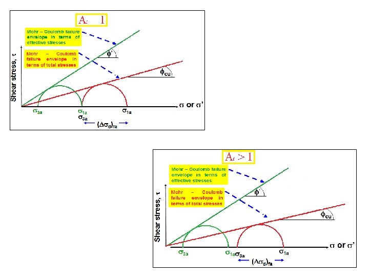
(Same as that obtained from CD test) NC OC Typically, the complete Mohr failure envelopes are determined by tests on several specimens consolidated over the working stress range of the field problem. The break in the total stress envelope (point z) occurs roughly at twice ’p for typical clays.

Notes on CU test • Shear Strength parameters in terms of total stresses are C and or Ccu and cu • Shear Strength parameters in terms of effective stresses are C’ and ’. • If the specimen tends to contract or consolidate during shear, then the induced p. w. p. is +ve. This is in loose sand N. C. clay. • If the specimen tends to EXPAND or swell during shear, the u decreases and may be –ve. This occurs in Dense sand OC clay. • Since the shear strength is controlled by the effective stress in the specimen at failure, the Mohr failure hypothesis is valid in terms of effective stresses only. Hence, the point of tangency of effective M-C failure envelope to the Mohr circle of effective stress is used to define f. • It is tacitly assumed that the Mohr-Coulomb strength parameters in terms of effective stresses determined by CU tests with pore pressure measurements would be the same as those determined by CD tests. We used the same symbols, C’ and ’ for the parameters determined both ways.

Some practical applications of CU analysis for clays o CU strengths are used for stability problems where the soils have first become fully consolidated and are at equilibrium with the existing stress system o Then, for some reasons, additional stresses are applied quickly with no drainage occurring. o Practical examples include 1. Embankment constructed rapidly over a soft clay deposit Soft clay = in situ undrained shear strength

2. Rapid drawdown behind an earth dam. No drainage of the core = Undrained shear strength of clay core Core 3. Rapid construction of an embankment on a natural slope = In situ undrained shear strength

Disadvantages of CU Test o It requires the measurement of u which is not an easy task and requires a great deal of care. o The sample cannot be assured to be fully saturated. o Effect of rate of loading. The stress-deformation and strength response of clay soils is rate-dependent; that is, usually the faster you load a clay, the stronger it becomes. o There are two objectives that are incompatible. o The rate of loading in one hand shall be slow that the proper pressures measured at the ends of the specimen are the same as those occurring in the vicinity of the failure plane. o On the other hand, the rate of loading in the field may be quite rapid, and therefore for correct modeling of the field situation, the rate of loading in the laboratory sample should be comparable.

EXAMPLE 1 A normally consolidated clay was consolidated under a stress of 150 k. Pa, then sheared undrained in axial compression. The principal stress difference at failure was 100 k. Pa, and the induced pore water pressure at failure was 88 k. Pa. Determine: a. The Mohr-Coulomb strength parameters in terms of both total and effective stresses analytically and graphically. b. The theoretical angle of the failure plane in the specimen. 3 =150 k. Pa 1 =150 +100 =250 k. Pa ’ 3 = 150 -88 =62 k. Pa ’ 1 = 250 -88 =162 k. Pa Sin = 100/(250+150)… > =14. 5 o Sin ’ = 100/(162+62)… > = 26. 5 o f = 45+ ’ /2 = 58 o Note: 200 150 27 o 100 15 o 50 58 o 50 100 150 200 250 300 • Failure plane is obtained from effective Mohr circle • Measuring p. w. p. makes it possible to obtained effective strength parameters

EXAMPLE 2 The shear strength of a normally consolidated clay can be given by the equation f = tan 27°. Following are the results of a consolidatedundrained test on the clay. • Chamber-confining pressure = 150 k. N/m 2 • Deviator stress at failure = 120 k. N/m 2 a. Determine the consolidated-undrained friction angle b. Pore water pressure developed in the specimen at failure 3 =150 k. N/m 2 1 =150 +120 =270 k. N/m 2 Sin = (270 -150)/(270+150)…. > =16. 6 o SIN ' = ( '1 - '3) / ( '1 + '3) But deviatoric stress of total and effective are always equal, hence '1 - '3 = 120 Sin 27 = 120/( '1+ '3) hence ( '1+ '3) = 120/sin 27 = 264. 3 k. Pa The difference between the center of total and effective Mohr circles is equal to u, or u = ( 1+ 3)/2 –( '1 - '3)/2 = (270+150)/2 –(264. 3)/2 Hence u = 77. 85 k. Pa

Topics q Introduction q Basic Principles q Components of Shear Strength of Soils q Normal and Shear Stresses on a plane q Mohr-Coulomb Failure Criterion q Laboratory Shear Strength Testing • Direct Shear Test • Triaxial Compression Test (UU Test) • Unconfined Compression Test q Field Testing (Vane Test) q Stress Path

III. Unonsolidated Unrained Test (UU Test) Piston (to apply deviatoric stress) O-ring Soil sample Perspex cell impervious membrane Porous stone Water Pore pressure or volume change Cell pressure Back pressure pedestal Closed all along the UU test

Stress conditions for the unconsolidated undrained test = Total, + Neutral, u Step 1: After application of cell pressure ’ 3 = 3 – uc = 0 C = 3 No drainage Effective, ’ C = 3 = + uc ’ 3 = 3 – uc = 0 Step 2: During application of axial load No drainage ’ 1 = 3 + d - uc ± ud 3 + d 3 uc ± ud = + Step 3: At failure ’Vf = 3 + f - uc ± udf = ’ 1 f 3 + f No drainage 3 ’ 3 = 3 - uc ± ud = u c± udf = ’hf = 3 - uc ± udf = ’ 3 f

Shear strength parameters o Three identical saturated soil samples are sheared to failure in UU triaxial tests. Each sample is subjected to a different cell pressure. No water can drain at any stage. At failure the Mohr circles are found to be as shown. Failure envelope, u = 0 cu 3 a 3 b 1 a 3 c 1 b 1 c f o All tests for fully saturated clays, which are assumed to be at the same void ratio (density) and water content, and consequently they will have the same shear strength since there is no CONSOLIDATION allowed.

Notes on UU TEST o Drainage is not allowed both during the application of the confining pressure 3 and during shearing. o The test specimen is sheared to failure by the application of deviator stress, d, and drainage is prevented. o Because of the application of chamber confining pressure 3, the pore water pressure in the soil specimen will increase by uc. o A further increase in the pore water pressure (ud) will occur because of the deviator stress application. o Usually u is not measured in this test. This test is total stress test. Analysis is in terms of gives Cu and u. o The added axial stress at failure ( d)f is practically the same regardless of the chamber confining pressure.

o All Mohr circles at failure will have the same diameter and the Mohr failure envelope will be a horizontal straight line and hence is called a = 0 condition with = su = constant. o f = cu = su is called undrained shear strength and is equal to the radius of the Mohr’s circle. o The =0 concept is applicable to only saturated clays and silts. o Since drainage is not allowed at any stage the test can be performed very quickly. So it is called Quick test or just Q-test. (10 -20 mins. ) o Typically, stress-strain curves for UU test are not different from CU and CD stress-strain curves for the same soils. o Intact specimens are required for this test, so it is conducted usually on clay samples.

Effective and total stress Mohr circles o If u is measured, although it is not measured in this test, then the effective stresses can be estimated and Mohr circle for that is drawn. o The deviator stress ( d)f to cause failure is the same as long as the soil is fully saturated and fully undrained during both stages of the test. o The total and effective Mohr circles are displaced horizontally by the pore pressure, u.

Effective stress Mohr’s circle at failure o The different total stress Mohr circles with a single effective stress Mohr circle indicate that the pore pressure is different for each sample. o As discussed previously increasing the cell pressure without allowing drainage has the effect of increasing the pore pressure by the same amount ( u = c) with no change in effective stress. o The change in pore pressure during shearing is a function of the initial effective stress and the moisture content. As these are identical for the three samples an identical strength is obtained.

Why does f is the same for all specimens? o There is only ONE UU effective stress Mohr Circle at failure, no matter what the confining pressure. But why this is the case? Specimen I: at Failure No drainage uc + udf 3 + df 3 ’ 1 = 3 + d – uc - udf = ’ 3 = 3 - uc - udf + For fully saturated clays, B = 1 (hence, uc = 3) Specimen II: at Failure No drainage ’ 1 = 3 + 3+ d – uc - udf 3 + 3+ d 3 = uc + uc+ ud + ’ 3 = 3 + 3 - uc udf Because the effective confining pressure is the same for Specimen I and II.

Example In an unconsolidated undrained triaxial test the undrained strength is measured as 17. 5 k. Pa. Determine the cell pressure used in the test if the effective strength parameters are c’ = 0, Φ’ = 26º and the pore pressure at failure is 43 k. Pa. Analytical solution Two Eqs. Two unknowns Graphical solution

Remarks o It is often found that a series of undrained tests from a particular site give a value of u that is not zero (Cu not constant). If this happens either: • The samples are not saturated, or • The samples have different moisture contents o If the samples are not saturated analyses based on undrained behavior will not be correct. o The undrained strength Cu is not a fundamental soil property. If the moisture content changes so will the undrained strength. S < 100% 3 c 3 b S > 100% 1 c 3 a 1 b 1 a Effect of degree of saturation on failure envelope

Some practical applications of UU analysis for clays o Like the CD and CU tests, the UU strength is applicable to certain critical design situations in engineering practice. o These situations are where the engineering loading is assumed to take place so rapidly that there is no time for the induced pore water pressure to dissipate or for consolidation to occur during the loading period. o UU test simulates the short term condition in the field. Thus, Cu can be used to analyze the short term behavior of soils 1. Embankment constructed rapidly over a soft clay deposit Soft clay = in situ undrained shear strength

2. Large earth dam constructed rapidly with no change in water content of soft clay = Undrained shear strength of clay core Core 3. Footing placed rapidly on clay deposit = In situ undrained shear strength

Topics q Introduction q Basic Principles q Components of Shear Strength of Soils q Normal and Shear Stresses on a plane q Mohr-Coulomb Failure Criterion q Laboratory Shear Strength Testing • Direct Shear Test • Triaxial Compression Test • Unconfined Compression Test q Field Testing (Vane Test) q Stress Path

Unconfined Compression Test (UC Test) o This a special class or type of UU test. In this test the confining pressure 3 = 0. o Axial load is rapidly applied and at failure 3 = 0 and the value of 1 necessary to cause failure is called the Unconfined Compression Strength qu. Failure by shear Failure by Bulging

o Because the undrained shear strength is independent of the confining pressure as long as the soil is fully saturated and fully undrained, we have o The difference in qu between different tests will depend on the level of compaction for each sample. o Since we said that in UU test strength is independent of 3, theoretically the value of Cu obtained from unconfined compression test or UU test must be the same. In practice, however Cu from UC is slightly lower than that from UU test.

Notes o The effective stress conditions at failure are identical for both UU and UC tests. And if the effective stress conditions are the same in both tests, then the strengths will be the same. For this to be true the following assumptions must be satisfied. 1. The specimen must be 100% saturated. 2. The specimen must be intact and contains no defects. 3. The soil must be very fine (clays) 4. The specimen must be sheared rapidly to failure.

Comments on Triaxial Tests Three types of strength parameters (Consolidated-drained, consolidatedundrained, and unconsolidated undrained) were introduced. There use depends on drainage conditions.

Determination of P. W. P. During Undrained Loadings o In CE 382 we learned how to determine u for the case of hydrostatic loading and steady state seepage. o In the preceding Chapter we learned how to evaluate u in the case of consolidation (i. e. drained loading). o It is often necessary in engineering practice to be able to estimate just how much excess pore water pressure develops in undrained loading due to a given set of stress changes. o Consider what happens when we apply the hydrostatic cell pressure c and prevent any drainage from occurring. • If the soil is 100% saturated, then we obtain a change in pore pressure u, numerically equal to the change in cell pressure c we just applied. In other words , the ratio u/ c equals 1.

After application of cell pressure Shear At failure For the case of full saturation B =1 u = 3 + A( 1 – 3)

Let us consider the case of UU test (we have p. w. p. all along the test) Step 1: Immediately after sampling Assuming S =100% 0 0 Step 2: After application of hydrostatic cell pressure C = 3 No drainage C = 3 uc = B 3 Increase of pwp due to increase of cell pressure Increase of cell pressure Skempton’s pore water pressure parameter, B Note: If soil is fully saturated, then B = 1 (hence, uc = 3)

Step 3: During application of axial load No drainage 3 + d 3 uc ± ud Increase of deviator stress Increase of pwp due to increase of deviator stress

Combining steps 2 and 3, uc = B 3 Total pore water pressure increment at any stage, u u = uc + ud Eq. (*) can also be expressed as o This is the well-known Skempton pore water pressure equation for relating the induced pore pressure to the changes in total stress in undrained loading.

Notes on P. W. P. parameters o The pore pressure parameter B expresses the increase in pore water pressure in undrained loading due to the increase in hydrostatic or cell pressure. o If the soil were less than 100% saturated, then the ratio of the induced u to the increase in cell pressure c would be less than 1. o The parameter B is very useful in the triaxial testing to determine if the test specimen is saturated. o The Skempton’s pore water pressure parameter “A” is a measure of how much pore pressure will change during shear phase. o Like the parameter B, the parameter A also is not constant. It is very dependent on, OCR, anisotropy, sample disturbance. o The parameter A can be calculated for the stress conditions at any strain up to failure, as well as at failure. o The Skempton pore pressure coefficients are most useful in engineering practice since they enable us to predict the induced pore pressure if we know or can estimate the change in the total stresses. Typical examples are in the design and construction of highway embankments and compacted earthfill dams.

Af B Degree of saturation The general range of values in most clay soils is as follows: • Normally consolidated clays: 0. 5 to 1 • Overconsolidated clays: - 0. 5 to 0 OCR

Topics q Introduction q Basic Principles q Components of Shear Strength of Soils q Normal and Shear Stresses on a plane q Mohr-Coulomb Failure Criterion q Laboratory Shear Strength Testing • Direct Shear Test • Triaxial Compression Test • Unconfined Compression Test q Field Testing (Vane Test) q Stress Path

Vane Shear Test o There are other techniques besides UU and UC tests from which Cu can be found. o One of the most versatile and widely used devices used for investigating undrained shear strength (Cu) is the VST. Applied Torque, T Bore hole (diameter = DB) Disturbed soil Rupture surface h > 3 DB) Vane T Vane H PLAN VIEW D Rate of rotation : 60 – 120 per minute Test can be conducted at 0. 5 m vertical intervals

o Since the test is very fast, Unconsolidated Undrained (UU) can be expected. o If T is the maximum torque applied at the head of the torque rod to cause failure, it should be equal to the sum of the resisting moment of the shear force along the side surface of the soil cylinder (Ms) and the resisting moment of the shear force at each end (Me). T = Ms + Me = Ms + 2 Me Ms – Shaft shear resistance along the circumference Cu Cu Me depends on the assumed distribution of shear strength mobilization at the ends of the soil cylinder. Cu Cu d/2 d/2 d/2 h

o In general, the torque, T, at failure can be expressed as b = 1/2 for triangular distribution b = 2/3 for uniform distribution b = 3/5 for parabolic distribution Remarks o The undrained shear strength obtained from a vane shear test also depends on the rate of application of torque T. o Bjerrum (1974) has shown that as the plasticity of soils increases, Cu obtained by vane shear tests may give unsafe results for foundation design. Therefore, he proposed the following correction. Cu(design) = l. Cu(vane shear) Where, l = correction factor = 1. 7 – 0. 54 log (PI) PI = Plasticity Index o Vane shear tests can be conducted in the laboratory and in the field during soil exploration. o In the field, where considerable variation in the undrained shear strength can be found with depth, vane shear tests are extremely useful.

Topics q Introduction q Basic Principles q Components of Shear Strength of Soils q Normal and Shear Stresses on a plane q Mohr-Coulomb Failure Criterion q Laboratory Shear Strength Testing • Direct Shear Test • Triaxial Compression Test • Unconfined Compression Test q Field Testing (Vane Test) q Stress Path

Stress Path o As we learned in the first part of this chapter, states of stress at a point in equilibrium can be represented by a Mohr circle in a - coordinate system. o Sometimes it is convenient to represent that state of stress by a stress point, which has the coordinates Stress point 3 1

o We often want to show successive states of stress which a test specimen or a typical element in the field undergoes during loading or unloading. o A simple case to illustrates stress paths is the common triaxial test in which 3 remain fixed as we increase 1. q 1 increasing This plane of maximum shear 45 o 3 p o There might be a confusion, especially if the stress path were complicated. Therefore it is simpler to show only the locus of the stress points. o This locus is called the stress path, and it is plotted on what is we call a p-q diagram. o A stress path is therefore a line that connects a series of points, each of which represents a successive stress state experienced by a soil specimen during the progress of a test. o Both p and q could be defined either in terms of total stresses or effective stresses

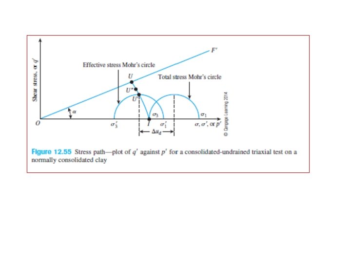
A modified failure envelope (Kf line). The straight line ID is referred to as the stress path in a q-p plot for a consolidated-drained triaxial test. Mohr’s circle at failure Mohr Coulomb failure envelope in terms of stress invariants

EXAMPLE A normally consolidated clay was consolidated under a stress of 150 k. Pa, then sheared undrained in axial compression. The principal stress difference at failure was 100 k. Pa, and the induced pore water pressure at failure was 88 k. Pa. The strain, deviatoric stress, and pore water pressure recorded during the test are listed in the Table below. Draw the total and effective stress paths for this test and determine the Mohr-Coulomb strength parameters.

e u 0. 25 49 35 0. 5 73 57 0. 75 86 72 1 94 79. 5 1. 25 100 88 1. 5 96 92 2 89 99 24. 5 36. 5 43 47 50 48 44. 5 115 93 78 70. 5 62 58 51 199 223 236 244 250 246 239 164 166 164. 5 162 154 140 139. 5 121 117. 5 112 106 95. 5 174. 5 186. 5 193 197 200 198 194. 5 q (k. Pa) ’ = 24. 8 o F’’ = 27. 5 o =14. 6 o = 15. 1 o p, p’ (k. Pa)

Question#3 (1 st Midterm, Fall 36 -37) A direct shear test was conducted on a specimen of dry sand (C = 0) with a normal stress of 190 k. N/m 2. Failure occurred at a shear stress of 120 k. N/m 2. The size of the sample tested was 50 mm X 25 mm (height). Determine: a. The angle of friction for the sand. b. The principal stresses at failure. c. The orientation of the plane of the maximum shear stress at failure. Solution tan ’ = 120/190 Hence ’ =32. 3 o From point F draw normal to the M-C Envelope. It intersects -axis at point C defining the center of Mohr circle. Draw Mohr circle such that its center is at point C and is tangent to the M-C envelope at point F. Get 1 and 3. 200 150 max =14 o =32. 3 o F POLE 100 50 0 1 =380 k. Pa 3 =125 k. Pa 50 100 C 150 200 250 300 350

Solution 1 = d + 3 = ( 1 – 3 ) + 150 ’ 3 = 3 - u = 150 - u ’ 1 - ’ 3 = 1 – 3 ’ 1 = ( 1 – 3) + ’ q = ( 1 – 3)/2 p’ = ( ’ 1 + ’ 3)/2 3 = ( 1 – 3) + 150 - u Values are listed in the table

Example 4 Given the stress shown on the element across. Required: a. Evaluate and when = 30 o. b. Evaluate 1 and 3. c. Determine the orientation of the major and minor principal planes. d. Determine the maximum shear stress and the orientation of the plane on which it acts.

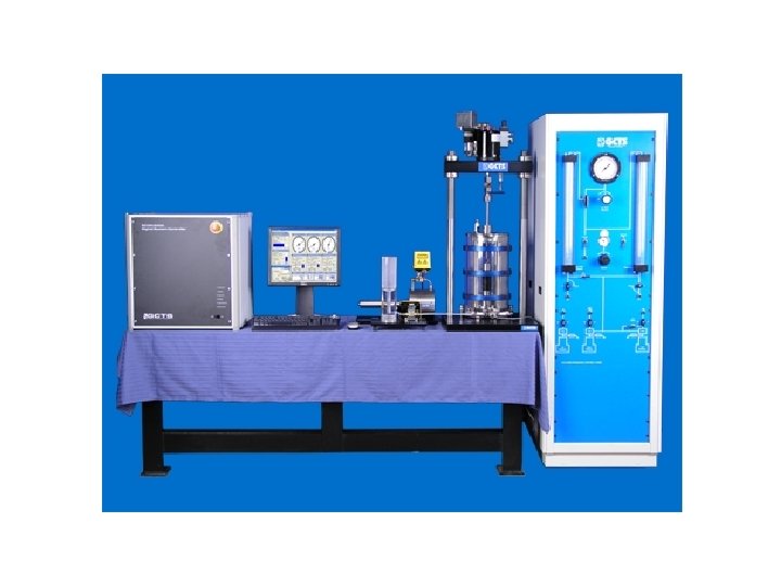
Triaxial Shear Test Device

Unconsolidated- Undrained test (UU Test) = Total, Step 1: Immediately after sampling 0 0 Neutral, u No drainage C -ur uc = -ur c (Sr = 100% ; B = 1) Step 3: During application of axial load C + No drainage Step 3: At failure No drainage C C + f C Effective, ’ HK Fig. 11. 38. It is too messy so I do not use it. ’V 0 = ur Instead simpler one ’h 0 = ur - ur Step 2: After application of hydrostatic cell pressure C + -ur c ± u ’VC = C + ur - C = ur ’ h = u r ’V = C + + ur - c ’ h = C + u r - c ’Vf = C + f + ur - c -ur c ± uf u u uf = ’ 1 f ’hf = C + ur - c uf = ’ 3 f

Unconsolidated Compression Test (UC Test) = Total, Neutral, u Step 1: Immediately after sampling 0 + Effective, ’ ’V 0 = ur ’h 0 = ur 0 - ur Step 2: During application of axial load No drainage C ’VC = C + ur - C = ur C -ur uc = -ur c ’h = ur (Sr = 100% ; B = 1) Step 3: During application of axial load No drainage C + C -ur c ± u ’h = C + ur - c ’Vf = C + f + ur - c Step 3: At failure No drainage ’V = C + + ur - c C + f C -ur c ± uf u u uf = ’ 1 f ’hf = C + ur - c uf = ’ 3 f