SOIL MECHANICSIICENG 2082 Lecture 01 SHEAR STRENGTH OF

SOIL MECHANICS-II(CENG 2082) Lecture 01: SHEAR STRENGTH OF SOILS Programme: BSc in Hydraulic and Water Resources Engineering Lecture by: Yonas B. (MSc. ) Faculty of Hydraulic and Water Resources Engineering Arba Minch Water Technology Institute

Objectives: ü How to determine the shear strength of soils ü Understands the differences between drained and undrained shear strength ü Determine the type of shear test that best simulates field conditions ü How to interpret laboratory and field test results to obtain shear strength parameters. ü Importance of Shear Strength for geotechnical engineering application

Output q When you complete this chapter, you should be able to: Ø Determine the shear strength of soils. Ø Understand the difference between drained and undrained shear strength. Ø Determine the type of shear test that best simulates field conditions. Ø Interpret laboratory and field test results to obtain shear strength parameters.

1. 1 Introduction Ø The shear strength of a soil mass is the internal resistance per unit area that the soil mass can offer to resist failure and sliding along any plane inside it. Ø The capability of the following comes from the soil shear strength : ü Support its own overburden & loading from structure ü Support Sustain slope in equilibrium

1. 1 INTRODUCTION… ü The safety of any geotechnical structure is dependent on the strength of the soil. If the soil fails, a structure founded on it can collapse, endangering lives and causing economic damages. ü Soils fail either in tension or in shear. However, in the majority of soil mechanics problems (such as bearing capacity, lateral pressure against retaining walls, slope stability, etc. ), only failure in shear requires consideration. ü The shear strength of soils is, therefore, of paramount importance to geotechnical engineers. ü The shear strength along any plane is mobilized by cohesion and frictional resistance to sliding between soil particles. The cohesion c and angle of friction of a soil are collectively known as shear strength parameters.

Shear failure of soils ü Shear Failure happens if the shear stress along the failure surface reaches the soil’s shear strength. ü Soil generally fail in shear. Embankment Strip footing Failure surface Mobilized shear resistance ü At failure, shear stress along the failure surface (mobilized shear resistance) reaches the shear strength.

Shear failure of soils… Embankment Failure Retai ning wall ü At failure, shear stress along the failure surface (mobilized shear resistance) reaches the shear strength.

Definitions of Key Terms ü Shear strength of a soil ( ) is the maximum internal resistance to applied shearing stresses. ü Angle of internal friction ( ) is the friction angle between soil particles. ü Cohesion (c) is a measure of the forces that cement soil particles. ü Undrained shear strength of a soil (Su) is the shear strength of a soil when sheared at constant volume.

1. 2 Coulomb’s Frictional Law ü The law for the shear strength of soil was propounded as early as 1773 by Charles Augustine Coulomb, a French military engineer. In fact Coulomb’s law for shear strength is considered the first milestone in classical soil mechanics. ü Recall Coulomb’s frictional law from your courses in statics and physics. If a block of weight W is pushed horizontally on a plane (Fig. 1. 1 a), the horizontal force (H) required to initiating movement is: H= *W; coef/t of static friction between the block and the horizontal plane. The coefficient of friction The angle between the resultant force R and the normal force N (Fig. 1. 1) is called the friction angle, .

1. 2 Coulomb’s Frictional Law Figure 1. 1: (a) Slip plane of a block. (b) A slip plane in a soil mass. ØIn terms of stresses, Coulomb’s law is expressed as: = * σ = *tan , since = tan-1( ) (1. 2) üCoulomb’s law requires the existence or the development of a critical sliding plane, also called slip plane or failure plane. In the case of the block the slip plane is at the interface between the block and the horizontal plane.

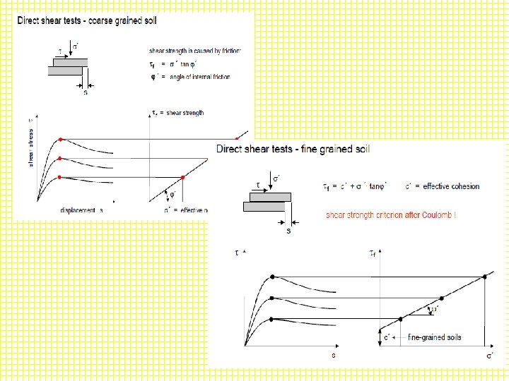
1. 2 Coulomb’s Frictional Law… n The limiting shear stress (soil strength) is given by : = c + tan where c = cohesion = angle of internal friction

1. 3 Mohr’s Circle for Stress ü The stress states at a point within a soil mass can be represented graphically by a very useful and widely used devise known as Otto Mohr’s circle for stress. ü For simplicity, we will consider a 2 D element with stresses as shown in Fig. 1. 2 a. Let’s draw Mohr’s circle. First, we have to choose a sign convention. ü In soil mechanics, compressive stresses and clockwise shear are generally assumed to be positive. We will also assume that z > x.

1. 3 Mohr’s Circle for Stress… Figure 1. 2: Stresses on a two-dimensional element and Mohr’s circle.

1. 3 Mohr’s Circle for Stress… Steps to draw Mohr’s circle for stresses: ü The two coordinates of the circle are ( z, zx) and ( x, zx). Recall from your strength of materials course that, zx=- zx for equilibrium. ü Plot these two coordinates on a graph of shear stress (ordinate) and normal stress (abscissa) as shown by A and B in Fig. 1. 2 b. Draw a circle with AB as the diameter. ü The circle crosses the normal stress axis at 1 and 3, where shear stresses are equal to zero. ü The stresses at these points are the major principal stress, 1 , and the minor principal stress, 3.

1. 3 Mohr’s Circle for Stress… The principal stresses are related to the plane stresses by the following relations: Major pr stress Minor pr stress tan 2 p=2* zx/( x- z) Maximum shear stress @ s= p+-45 The stresses on a plane oriented at an angle to the majo principal stress plane are: is measured in clockwise direction

EXAMPLE 1. 1 A sample of soil 100 mm× 100 mm is subjected to the forces shown in Fig. E 1. 1 a. Determine (a) ; (b) the maximum shear stress, and (c) the stresses on a plane oriented at 300 clockwise to the major principal stress plane.

Session 3; 1. 4 Mohr-Coulomb Failure Criterion 17

1. 4 Mohr-Coulomb Failure Criterion ü Coulomb (1776) suggested that the shear strength of a soil along a failure plane could be described by: ü Shear strength consists of two components: cohesive and frictional. Drained condition Un-Drained condition Mohr-Coulomb envelope f f tan c c f co nt ive hes ne mpo co frictional component f is the maximum shear stress the soil can take without failure, under normal stress of . 18

1. 4 Mohr-Coulomb Failure Criterion Figure 1. 5: Mohr-Coulomb failure criterion.

1. 4 Mohr-Coulomb Failure Criterion… ü Any point F at the failure plane represents the normal and shear stresses on a failure plane at a specified point in a soil. These stresses must also satisfy the equilibrium conditions at the point, which is represented by Mohr’s circle of stress. ü This implies that, at failure, Mohr’s circle of stress must be tangent to the line expressed by coulomb’s law of srtength. ü This condition known as the Mohr-Coulomb failure criterion is shown in Fig. 1. 5.

Mohr Coulomb failure criterion with Mohr circle of stress (Relation of stresses can be calculated Failure envelope in terms ’v = ’ 1 as) of effective stresses X ’h = ’ 3 F effective stresses B X is on failure A ’ O c’ ’ 3 (s’ 1 - s’ 3)/2 ’ 1 ’ c’ Cotf’ (s’ 1+ s’ 3)/2 Therefore, tan = op/adj= OB/AO =c’/AO AO= c’/ tan = c’ *cot

Mohr Coulomb failure criterion with Mohr circle of stress

Mohr Coulomb failure criterion… If the cohesion c’, is small or zero, then Eqs. (1. 15 to 1. 19) can be rearranged as follows: By rearranging Or

EXAMPLE 1. 2 q At a point in a soil mass, the total vertical and horizontal stresses are 240 k. Pa and 145 k. Pa respectively whilst the pore water pressure is 40 k. Pa. Shear stresses on the vertical and horizontal planes passing through this point are zero. ü Calculate the maximum excess pore water pressure to cause the failure of this point. ü What is the magnitude of the shear strength on the plane of failure? The effective parameters are c’ = 10 k. Pa and ɸ= 300. shear strength

1. 5 Drained and Undrained Shear strength Ø Drained condition occurs when the excess pore water pressure developed during loading of a soil dissipates, i. e. u=0, resulting in volume changes in the soil. ü Loose sands, normally consolidated clays and lightly overconsolidated clays tend to compress or contract, whilst dense sands and heavily overconsolidated (OCR > 2) clays tend to expand during drained condition. Effective stress Pore water pressure Effective stress

1. 5 Drained and Undrained Shear strength… Ø Undrained condition occurs when the excess pore water pressure cannot drain, at least quickly from the soil, i. e. u≠ 0. During undrained shearing, the volume of the soil remains constant. Ø If the specimen tends to compress or contract during shear, then the induced pore water pressure is positive. It wants to contract and squeeze water out of the pores, but it can not. ü Positive pore water pressures occur in loose sands, normally consolidated clays and lightly overconsolidated clays.

1. 5 Drained and Undrained Shear strength… ü If the specimen tends to expand swell during shear, the induced pore water pressure is negative. It wants to expand draw water into the pores, but it can not. Negative pore water pressures occur in dense sands and heavily overconsolidated (OCR > 2) clays. ü During the life of the geotechnical structure, called the long-term condition, the excess pore water pressure developed by a loading dissipates and drained condition applies. Clays usually take many years to dissipate the excess pore water pressure. ü During construction, and shortly after, called the short-term condition, soils with low permeability (fine-grained soils) do not have sufficient time for the excess pore water pressure to dissipate and undrained condition applies. ü The permeability of coarse-grained soils is sufficiently large that under static loading conditions the excess pore water pressure dissipates quickly. Consequently undrained condition does not apply to clean coarse-grained soils under static loading.

1. 5 Drained and Undrained Shear strength… Ø The shear strength of a fine-grained soil under undrained condition is called the undrained shear strength, S u. The undrained shear strength Su is the radius of Mohr’s total stress circle; that is:

Session 4; 1. 6 Laboratory Shear Strength Tests 29

1. 6 Laboratory Shear Strength Tests q Different methods are available for testing shear strength of soils in a laboratory. The following are the more commonly used testing methods: I. Direct shear test. II. Triaxial compression test. III. Unconfined compression test. To do what? Ø Determination of shear strength parameters of soils (c, f or c’, f’)

1. 6. 1 Direct Shear Test Ø ASTM D 3080 - Standard Test Method for Direct Shear Test of Soils Under Consolidated Drained Conditions Ø The direct shear test is the oldest and the simplest type of shear test. It was first devised by Coulomb (1776) for the study of shear strength. Ø The test is performed in a shear box, illustrated in Figure 1. 6. The box consists of two parts, one part fixed and the other movable. Ø Usually the box is a square of sides equal to 5/6 cm. The soil sample is placed in the box. Ø A vertical normal force N(at least 3; 1, 2, 3 kg) is applied to the top of the sample through a metal platen resting on the top part of the box. Ø Porous stones may be placed on the top and bottom part of the sample to facilitate drainage.

1. 6. 1 Direct Shear Test Figure 1. 6: Schematic of direct shear apparatus.

1. 6. 1 Direct Shear Test

Direct shear device

1. 61. Direct shear test… ü The sample is subjected to shearing stress at the plane of separation AA (Fig. 1. 6) by applying horizontal forces T. ü The horizontal force can be applied either at a constant speed (strain controlled test) or constant load (stress controlled test) until failure occurs in the soil. In most routine soil tests the strain controlled test is used. ü Failure is determined when the soil can not resist any further increment of horizontal force. ü The above procedure is repeated for several values (three or more) of normal forces.

1. 61. Direct shear test… ü By plotting the normal stresses and corresponding shear stresses from the results of such tests, a failure envelope is obtained as shown in Fig. 1. 7. ü Note that the normal stress σ=N/A, and the shear stress =T/A, where A is the cross-sectional area of the soil specimen. For example, if the normal and horizontal forces for the second test are represented by N 2 and T 2, respectively, the coordinate point for test 2 is given as (σ2=N 2/A, 2=T 2/A).

1. 61. Direct shear test… ü The corresponding Mohr’s circle for this case is shown in Fig. 1. 7 and the shear strength parameters and c could be measured directly(two point method). It is not possible to obtain other deformation parameters such Young’s modulus and Poisson’s ratio from direct shear test. Figure 1. 7: Plotted direct shear test results and a Mohr circle.

1. 61. Direct shear test… ü In direct shear test, drainage should be allowed through out the test because there is no way of sealing the specimen. ü In sands, due to their high permeability, dissipation of excess pore water pressure is immediate, and the test can be conducted quickly. ü In clayey soils full drainage may require long testing time to allow for dissipation of excess pore water pressure. Some practical engineers still attempt to perform undrained direct shear test in clayey soils by shearing the soil very quickly. However, this may lead to totally erroneous results.

1. 6. 1 Direct Shear Test… Advantages ü Test in inexpensive ü Fast and simple ü Easy to prepare for cohesion less samples Disadvantages ü Failure plane is forced to be horizontal(but not always) ü Cannot control drainage ü Stress concentrations at the sample boundaries ü Uncontrolled rotation of principal planes and stresses

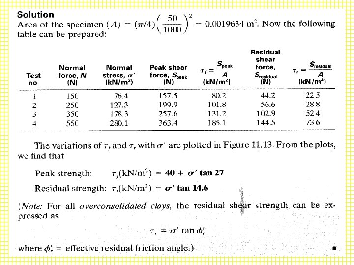
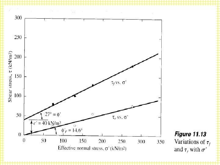
1. 6. 1 Direct Shear Test/example

1. 6. 1 Direct Shear Test Maximum shear Tmax 1= 45. 82 k. N/m 2

1. 6. 1 Direct Shear Test

Example A direct shear test on remolded sand soil has the following observation at time failure; normal stress of 288 N shear load of 173 N. The cross sectional area of sample is 36 cm 2. then determine shear parameters, principal stresses at zone of failure. Solution: Shear stress; f= 173/36=4. 8 k. N/cm 2=48 k. N/m 2 (at failure pt) Normal stress; σf = 288/36=8 k. N/cm 2=80 k. N/m 2(at failure pt) 1. Put failure point(σf, f) on the Mohr’s circle coordinate 2. Connect failure point and coordinate origin; since soil is sand(c=0) 3. Then determine ɸ by compus( is 310) 4. Rotate ɸ degree to counter clockwise from vertical line passing through failure point; to have center of circle. 5. Having center, draw Mohr circle with radius C to F 6. Then find principal stresses

Example DS

Session 4; 1. 6. 2 Triaxial Compression Test 48

vc + Laboratory tests Simulating field conditions in the laboratory 0 vc 0 0 0 Representative soil sample taken from the site t s e l t hc a i x a Tr vc + vc Di re hc hc ct sh ea vc Step 1 Set the specimen in the apparatus and apply the initial stress condition r t es t vc Step 2 Apply the corresponding field stress conditions

1. 6. 2 Triaxial Compression Test ü Triaxial Compression Test was introduced by Casagrande and Terzaghi in 1936 ü A widely used apparatus to determine the shear strength parameters and the stress -strain behavior of soils is the triaxial apparatus; as shown in Fig. 1. 8. ü The test is designed to as closely as possible mimic actual field or “in situ” conditions of the soil. Advantage over DST ü More versatile ü Drainage can be well controlled ü No rotation of principal plane and stresses ü Failure plane can occur anywhere Triaxial tests are run by: − saturating the soil − applying the confining stress (called σ3) − Then applying the vertical stress (sometimes called the deviator stress) until failure

1. 6. 2 Triaxial Compression Test Principles of triaxial compression test(TC) ü Is used to measure shaer strength of soil under controlled drainage condition ü Cylindrical soil specimen is enclosed and subjected to confining fluid/air pressure and then loaded axially to failure. ü Test is called triaxail b/c of three principal stresses are known and controlled.

Principles of triaxial compression test(TC). .

1. 6. 2 Triaxial Compression Test ü The soil sample(undistrubed) is protected by a thin rubber membrane and is subjected to pressure from water that occupies the volume of the chamber. This confining water pressure (also called radial pressure) enforces a condition of equality on two of the total principal stresses, i. e. 2= 3. Vertical or axial stresses are applied by a loading ram (plunger), and therefore, the total major principal stress, σ1 is the sum of the confining pressures and the deviatoric stress (σ1=σ3+∆σ) applied through the ram. ü In a traditional triaxial compression test, the confining pressure σ3 is kept constant whilst the major principal stress 1 is increased incrementally by the loading ram until the sample fails.

Triaxial Test Equipment

Part of machine 1. 6. 2 Triaxial Compression Test

Triaxial Shear Test Specimen preparation (undisturbed sample) Edges of the sample are carefully trimmed Setting up the sample in the triaxial cell

1. 6. 2 Triaxial Compression Test; Triaxial cell

1. 6. 2 Triaxial Compression Test Figure 1. 8: Schematic diagram of a triaxial compression apparatus (Budhu, pp. 225).

Triaxial Shear Test Piston (to apply deviatoric stress) Failure plane O-ring impervious membrane Soil sample at failure Perspex cell Porous stone Water Cell pressure Back pressure Pore pressure or pedestal volume change

1. 6. 2 Triaxial Compression Test ü The triaxial apparatus is versatile because we can ① independently control the applied axial and radial loads, ② conduct tests under drained and undrained conditions, and ③ control the applied displacements or stresses. ü Recorded measurements include deviatoric stress at different stages of the test, vertical displacement of the ram, volume change and pore water pressure.

1. 6. 2 Triaxial Compression Test Ø The average stresses and strains on a soil sample in a triaxial compression apparatus are as follows: Axial stress Axial strain Volumetric strain Deviatoric stress Radial strain Deviatoric strain ü where Pz is the axial load on the ram (from proving reading), A is the cross-sectional area of the soil sample at any stage of test, r 0 is the initial radius of the soil sample, r is the change in radius, V 0 is the initial volume, is the change in volume, H 0=ho is the initial height, and Z=∆h is the change in height.

Area correction for the determination of additional axial load/Deviatoric stress(∆σ) • Where A 0 (= *ro 2) is the initial cross-sectional area and H is the current height of the sample.

Types of Triaxial Tests ü Depending on whether drainage is allowed or not during v initial isotropic cell pressure application/ consolidation phase, and v shearing(during loading valve is open or not) , ü Having these; there are three special types of triaxial tests that have practical significances. They are: Consolidated Drained (CD) test(S-test) Consolidated Undrained (CU) test(R-test) Unconsolidated Undrained (UU) test(Q-test) 63

Types of Triaxial Tests c Step 2 Step 1 c c deviatoric stress ( = q) c c c+ q c Under all-around cell pressure c Is the drainage valve open? yes Consolidated sample no Shearing (loading) Is the drainage valve open? yes no Unconsolidated Drained Undrained sample loading

A. Consolidated – Drained Triaxial Test ü The purpose of a CD test is to determine the drained shear strength parameters ’ and c’. ü The specimen is saturated ü Confining stress (σ3) is applied (stage 1) § This squeezes the sample causing volume decrease § Drain lines kept open and must wait for full consolidation (u = 0) to continue with test ü Once full consolidation is achieved, normal stress applied to failure with drain lines still open (stage 2) § Normal stress applied very slowly allowing full drainage and full consolidation of sample during test (u = 0) ü Test can be run with varying values of σ3 to create a Mohrs circle and to obtain a plot showing c’ and φ’ 65

A. Consolidated – Drained Triaxial Test… ü Test can also be run such that σ3 is applied allowing full consolidation, then decreased (likely allowing some swelling) then the normal stress applied to failure simluating overconsolidated soil. ü In the CD test, the total and effective stress is the same since u is maintained at 0 by allowing drainage; means you are testing the soil in effective stress conditions ü Applicable in conditions where the soil will fail under a long term constant load where the soil is allowed to drain (long term slope stability) 66

Deviator stress, d CD tests How to determine strength parameters c and ( d)fc 1 = 3 + ( d)f Confining stress = 3 c Confining stress = 3 b 3 Confining stress = 3 a ( d)fb ( d)fa Shear stress, Axial strain Mohr – Coulomb failure envelope 3 a 3 b 3 c 1 a ( d)fb 1 c or ’

1. CD data and analysis Example 1 (CD) ∆V=0 2. σ1 determination

3. Mohr circle 4. CD Triaxial Test on Sand -Figure

Example 2 (CD)

Example 3 (CD)

Example 4 (CD) ü A consolidated drained triaxial test was conducted on granuar soil. At failure ratio of major to minor principal stresses is 4. the effective minor stress at failure was 100 k. N/m 2. compute ɸ’ and deviatoric stress. Solution: 1. ɸ’=37 2. σ1’-σ3’=∆σ=300 k. N/m 2

Example 5 (CD) Triaxial compression test of two lots of tests , the shearing resistance of which is governed by coulomb’s law( = c + tan ) Test 1; σ1’=800 k. N/m 2 σ3’=200 k. N/m 2 Test 2; σ1’=1050 k. N/m 2 σ3’=350 k. N/m 2 Ø Then determine shear parameters of given soil. Solution: 1. Draw Mohr circle first for above two tests 2. Determine φ by 3. Draw tangent to two circles having φ 4. Determine C’ by Ø

B. Consolidated Undrained (CU) Test ü The purpose of a CU test is to determine both the undrained (cu, ɸu ) and drained (c’, ’) shear strength parameters; Eu and E’ are also obtained from this test. ü The CU test is conducted in a similar manner to the CD test except that after isotropic consolidation, the axial load is increased under undrained condition and the excess pore water pressure is measured. ü As explained in section 1. 5, the excess pore pressure developed during shear can either be positive or negative. This happens because the sample tries to either contract or expand during shear. ü Positive pore pressures occur in loose sands and normally consolidated clays. Negative pore pressures occur in dense sands and heavily overconsolidated clays.

B. Consolidated Undrained (CU) Test… ü The CU test is the most popular triaxial test because you can obtain both drained and undrained shear strength parameters, and most tests can be completed within a few minutes after consolidation compared with more than a day for a CD test. ü Fine-grained soils with low permeability must be sheared slowly to allow the excess pore water pressure to equilibrate throughout the test sample. The results from CU tests are used to analyze the stability of slopes, foundations, retaining walls, excavations and other earthworks. ü For remolded and normally consolidated clays, the cohesion c’ parameter from a CU test is also essentially very small and can be assumed to be zero.

B. Consolidated – Undrained Triaxial Test ü The specimen is saturated ü Confining stress (σ3) is applied § This squeezes the sample causing volume decrease § Again, must wait for full consolidation (u = 0) ü Once full consolidation is achieved, drain lines are closed (no drainage for the rest of the test), and normal stress applied to failure § Normal stress can be applied faster since no drainage is necessary (u not equal to 0) ü Test can be run with varying values of σ3 to create a Mohrs circle and to obtain a plot showing c & φ /c’ & φ’ ü Applicable in situations where failure may occur suddenly such as a rapid drawdown in a dam or levee ü This test can simulates long term as well as short term shear strength for cohesive soils if pore water pressure is measured during 76 the shearing phase

Triaxial Compression Test Deviator Stress 1 - Consolidated Undrained Test (CU) Step 1 2 Step 2 Failure e 1 = + 2 Confining Pressure 2 2 2 = c 2 cu 2 2 2 + n 2 1 - 2 fu tan 1 1 - 2 1 n

CU for c & φ /c’ & φ’ Over-consolidated clav n n ta = Normally consolidated clav n = ta c + n Fig: Effective stress failure envelope for Normally/overconsolidated clav

Example (cu) Soil sample under triaxial compresion test has the following observations: change in length is 0. 04 cm(h=16 cm), area of sample Ao=40 cm 2, confining stress of 200 kpa and additional loading of 0. 8 k. N. Then calculate: i. Deviatoric stress ii. Principal stresses(σ1 & σ3) Solution: A=Ao/(1 -εa) but εa=∆h/ho=0. 04/16=0. 002 A=40/(1+0. 002)=40. 1 cm 2=0. 004 m 2 ∆σ=0. 8/0. 004=199. 5 kpa Σ 1=200+199. 5=399. 5 kpa Σ 3=200 kpa

Example CU

C. Unconsolidated Undrained (UU) Test ü The purpose of a UU test is to determine the undrained shear strength (Su) of a saturated soil. ü The UU test consists of applying a cell pressure to the soil sample without drainage of pore water followed by increments of axial stress. ü The cell pressure is kept constant and the test is completed very quickly because in neither of the two stages – consolidation and shearing – is the excess pore pressure allowed to drain. In the UU test, pore water pressures are usually not measured.

c. Unconsolidated – Undrained Test ü The specimen is saturated ü Confining stress (σ3) is applied without drainage or consolidation (drains closed the entire time) ü Normal stress then increased to failure without allowing drainage or consolidation ü This test can be run quicker than the other 2 tests since no consolidation or drainage is needed. Test can be run with varying values of σ3 to create a Mohrs circle and to obtain a plot showing c and φ ü UU test simulates short term shear strength for cohesive soils. ü Applicable in most practical situations – foundations for example. ü This test commonly shows a φ = 0 condition 82

Example(UU) Ø UU triaxial test was conducted on soil sample and has following laboratory observations were taken; confining stress of 810 k. N/m 2, vertical additional stress of 62. 50 k. N/m 2 and PWP = 31. 25 k. N/m 2 i. Total principal stresses ii. Effective principal stresses iii. Shear strength parameters Solution: ü σ1=810+62. 5=872. 5 k. N/m 2, σ3=810 k. N/m 2 ü Σ 1’=872. 5 -31. 25=…. k. N/m 2, σ3’=810 -31. 25=…. k. N/m 2 ü SU=CU=(σ1 -σ3)/2=810 k. N/m 2 =(σ1’-σ3’)/2= …. k. N/m 2

Failure Conditions Unconsolidated Undrained (UU or Q) ü – Failure that occurs rapidly during or shortly after construction. Consolidated Undrained (CU or R) ü – Failure that occurs rapidly after the soil has had time to consolidate. Consolidated Drained (CD or S) ü – Failure that occurs slowly after the soil has had time to consolidate. 84

Fig: Mohr circle for ɸ=0 soil UU test Fig: Mohr circle for C =0 soil UU test

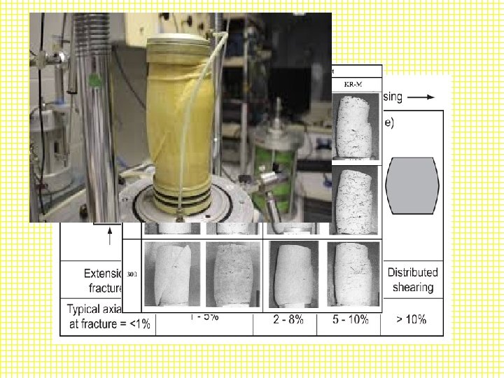
Triaxial failure modes on specimens plastic failure type Brittle failure type

Comparison of Shear Strengths 88

Cell pressure and Backpressure ü Backpressure is a technique used for saturating soil specimens. It is accomplished by applying water pressure u 0 within the specimen, and at the same time changing the cell pressure of an equal amount. ü Therefore, the net confining pressure remains unchanged. ü Backpressuring has no influence on the calculations. In most cases, a backpressure of 300 k. Pa is sufficient to ensure specimen saturation and it should be applied in steps as shown in the table below.

Session 5; 1. 6. 3 Unconfined Compression (UC) Test 90

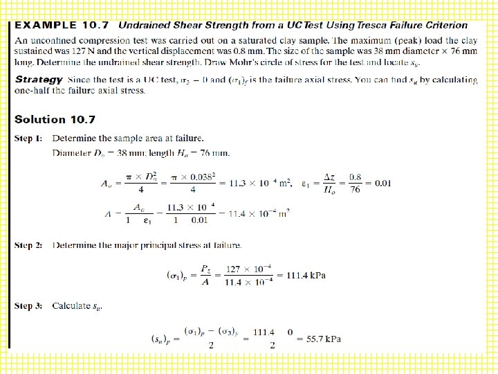
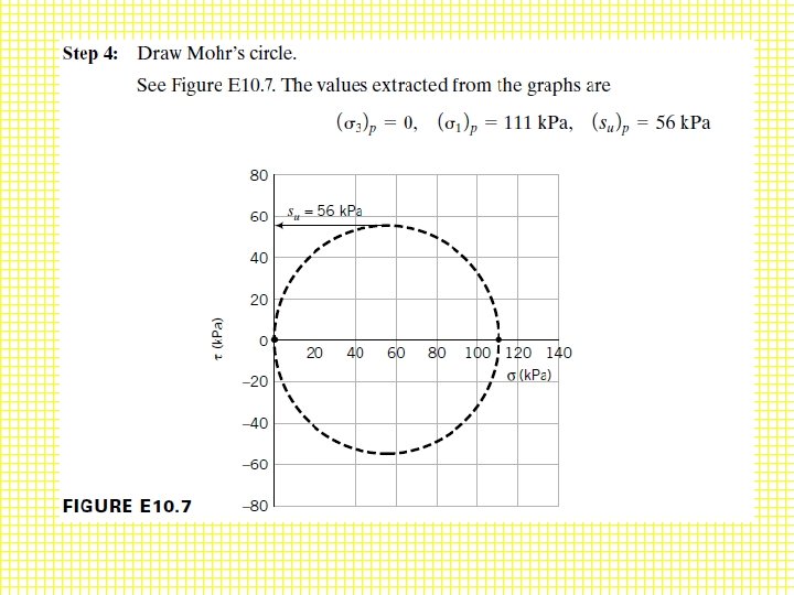
1. 6. 3 Unconfined Compression (UC) Test ü The UC test is the simplest and quickest test used to determine the shear strength of a cohesive soil. ü An undisturbed or remolded sample of cylindrical shape, about 38 mm in diameter and 76 mm in height is subjected to uniaxial compression until the soil fails. ü Since the sample is laterally unconfined, only cohesive soils can be tested. The sample is tested quickly and there is no drainage. ü Therefore, it is a special case of the UU test in which 3=0. However, rather than in a triaxial cell, the test is performed in a mechanical apparatus specially manufactured fro this purpose. ü See Figure 1. 9 shows an unconfined compression test apparatus.

1. 6. 3 Unconfined Compression (UC) Test. . Figure 1. 9: (a) Direct shear test apparatus, (b) UC test apparatus

Unconfined Compression Test… ü The specimen is not placed in the cell ü Specimen is open to air with a σ3 of 0 ü Test is similar to concrete compression test, except with soil (cohesive – why? ) ü Applicable in most practical situations – foundations for example. ü Drawing Mohrs circle with σ3 at 0 and the failure (normal) stress σ3 defining the 2 nd point of the circle – often called qu in this special case ü c becomes ½ qu of the failure stress 93

Unconfined Compression Test Deviator Stress Failure e = cu Cu = qu/2 1 qu = Unconfined compressive strength Cu = Unconfined shear strength qu = 1 n

Example UC Unconfined compressive test of soft clay data length of sample L=10 cm, initial area=10 cm 2, load at failure P=0. 2 k. N. Compression at failure ∆L=0. 2 cm. Then determine unconfined compressive strength and shear strength of soil sample. Solution: A=Ao/(1 -εa) but εa=∆h/ho=2/10=0. 2 A=10/(1 -0. 2)=12. 5 cm 2=(12. 5/10000)m 2 i. ∆σ=0. 2/(12. 5/10000)=160 kpa=qu(unconfined compressive strength) ii. =qu/2=80 kpa

1. 7 Field Tests for shear ü Sampling disturbances and sample preparation for laboratory tests significantly affect the shear strength parameters. Consequently, a variety of field tests have been developed to obtain more reliable soil shear strength parameters by testing soils in-situ. 1. 7. 1 Shear Vane ü In soft and saturated clays, where undisturbed specimen is difficult to obtain, the undrained shear strength is measured using a shear vane test. A diagrammatic view of the shear vane apparatus is shown in Fig. 1. 20. It consists of four thin metal blades welded orthogonally (900) to a rod where the height H is twice the diameter D (Fig. 1. 20). Commonly used diameters are 38, 50 and 75 mm.

Figure 1. 20: Shear vane apparatus. ü The vane is pushed into the soil either at the ground surface or at the bottom of a borehole until totally embedded in the soil (at least 0. 5 m). A torque T is applied by a torque head device (located above the soil surface and attached to the shear vane rod) and the vane is rotated at a slow rate of 60 per minute. As a result, shear stresses are mobilized on all surfaces of a cylindrical volume of the soil generated by the rotation. The maximum torque is measured by a suitable instrument and equals to the moment of the mobilized shear stress about the central axis of the apparatus. The undrained shear strength is calculated from:

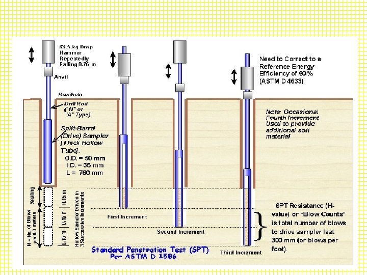
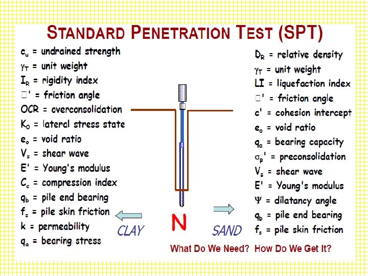
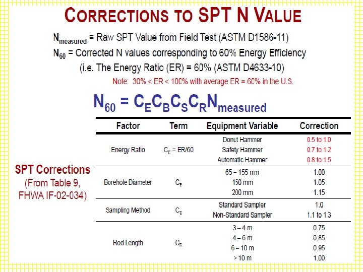
1. 7. 2 Standard Penetration Test (SPT) ü The Standard Penetration Test (SPT) was developed around 1927 and it is perhaps the most popular field test performed mostly in coarse grained (or cohesionless) soils. The SPT is performed by driving a standard split spoon sampler into the ground by blows from a drop hammer of mass 64 kg falling 760 mm (Fig. 1. 21). ü The sampler is driven 150 mm into the soil at the bottom of a borehole, and the number of blows (N) required to drive it an additional 300 mm is counted. ü The number of blows N is called the standard penetration number.

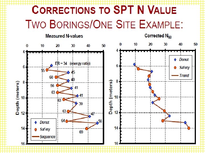
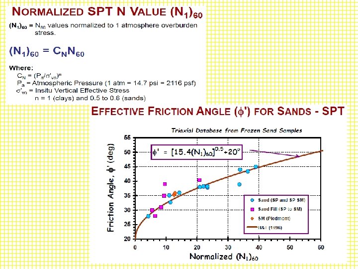
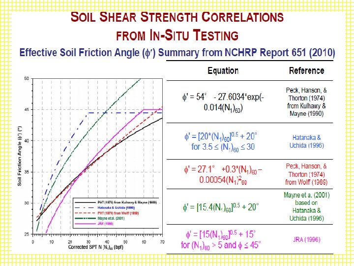
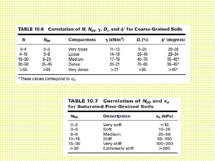
Figure 1. 21: Standard Penetration Test (Budhu, 248) ü Various corrections are applied to the N values to account for energy losses, overburden pressure, rod length, and so on. It is customary to correct the N values to a rod energy ratio of 60%. The rod energy ratio is – the ratio of the energy delivered to the split spoon sampler to the free falling energy of the hammer. The corrected N values are denoted as N 60. The N value is used to estimate the relative density, friction angle, and settlement in coarse grained soils. The test is very simple, but the results are difficult to interpret.

1. 8 Cone Penetration Test (CPT) ü The Cone Penetrometer Test (CPT) is an in situ test used for subsurface exploration in fine and medium sands, soft silts and clays. The apparatus consists of a cone with a 35. 7 mm end diameter, projected area of 1000 mm 2 and 600 point angle (Fig. 1. 22) that is attached to a rod. An outer sleeve encloses the rod. Figure 1. 22: CPT apparatus (Budhu, 250)

1. 8 Cone Penetration Test (CPT)… ü The thrusts required to drive the cone and the sleeve 80 mm into the ground at a constant rate of 10 mm/s to 20 mm/s are measured independently so that the end resistance or cone resistance and side friction or sleeve resistance may be estimated separately. ü A special type of the cone penetrometer, known as piezocone has porous elements inserted into the cone or sleeve to measurements. allow for pore water pressure

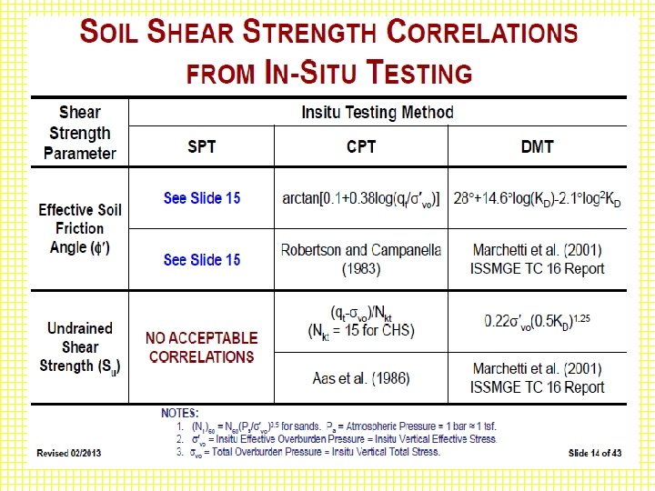
ü The cone resistance qc is normally correlated with the undrained shear strength. Several adjustments are made to qc. One correlation equation is where Nk is a cone factor that depends on the geometry of the cone and the rate of penetration. Average values of Nk as a function of plasticity index can be estimated from ü Results of cone penetrometer tests have been correlated with the peak friction angle. A number of correlations exist. Based on published data for sand (Robertson and Campanella, 1983), you can estimate ɸ’p using

References: 1. Das, Braja, Principles of Geotechnical Engineering, 5 th ed. , Brooks/Cole, 2002. 2. Budhu M. (2000), Soil Mechanics and Foundations, Wiley and Sons. 3. Lambe, T. W. , Whitman, R. V. (1999), Soil Mechanics, John Wiley & Sons Inc. 4. Teferra, A. & Mesfin, L. , Soil Mechanics, AAU 5. Craig, R. F. (2004), Craig's Soil Mechanics, 7 th edition, Taylor & Francis. 6. Bowles, J. E. , 1996. Foundation Analysis and Design, Joseph E. Bowles, Mc. Graw-Hill.

THANK YOU!