Simulating the Atmospheric Fate and Transport of Mercury

Simulating the Atmospheric Fate and Transport of Mercury using the NOAA HYSPLIT Model Mark Cohen, Roland Draxler and Richard Artz NOAA Air Resources Laboratory 1315 East West Highway, R/ARL, Room 3316 Silver Spring, Maryland, 20910 Presentation at the NOAA Atmospheric Mercury Meeting November 14 -15, 2006, Silver Spring MD

methodology 2

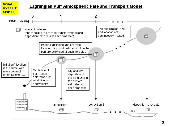
NOAA HYSPLIT MODEL Lagrangian Puff Atmospheric Fate and Transport Model 0 1 2 TIME (hours) The puff’s mass, size, and location are continuously tracked… = mass of pollutant (changes due to chemical transformations and deposition that occur at each time step) Phase partitioning and chemical transformations of pollutants within the puff are estimated at each time step Initial puff location is at source, with mass depending on emissions rate Centerline of puff motion determined by wind direction and velocity Dry and wet deposition of the pollutants in the puff are estimated at each time step. deposition 1 deposition 2 deposition to receptor lake 3

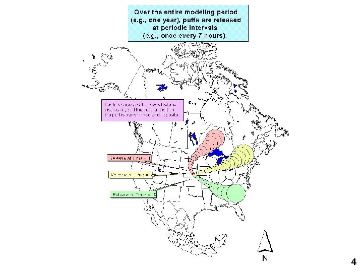
4

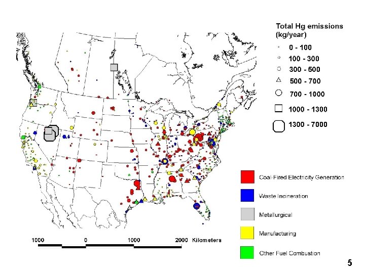
5

• In principle, we need do this for each source in the inventory • But, since there are more than 100, 000 sources in the U. S. and Canadian inventory, we need shortcuts… • Shortcuts described in Cohen et al Environmental Research 95(3), 247 -265, 2004 6

Cohen, M. , Artz, R. , Draxler, R. , Miller, P. , Poissant, L. , Niemi, D. , Ratte, D. , Deslauriers, M. , Duval, R. , Laurin, R. , Slotnick, J. , Nettesheim, T. , Mc. Donald, J. “Modeling the Atmospheric Transport and Deposition of Mercury to the Great Lakes. ” Environmental Research 95(3), 247 -265, 2004. Note: Volume 95(3) is a Special Issue: "An Ecosystem Approach to Health Effects of Mercury in the St. Lawrence Great Lakes", edited by David O. Carpenter. 7

• For each run, simulate fate and transport everywhere, but only keep track of impacts on each selected receptor (e. g. , Great Lakes, Chesapeake Bay, etc. ) • Only run model for a limited number (~100) of hypothetical, individual unit-emissions sources throughout the domain • Use spatial interpolation to estimate impacts from sources at locations not explicitly modeled 8

Spatial interpolation Impact of source 4 estimated from weighted average of impacts of nearby explicitly modeled sources 1 2 Impacts from Sources 1 -3 are Explicitly Modeled RECEPTOR 4 3 9

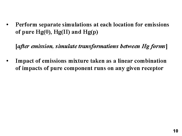
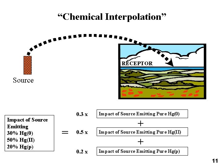
• Perform separate simulations at each location for emissions of pure Hg(0), Hg(II) and Hg(p) [after emission, simulate transformations between Hg forms] • Impact of emissions mixture taken as a linear combination of impacts of pure component runs on any given receptor 10

“Chemical Interpolation” RECEPTOR Source Impact of Source Emitting 30% Hg(0) 50% Hg(II) 20% Hg(p) = 0. 3 x Impact of Source Emitting Pure Hg(0) 0. 5 x Impact of Source Emitting Pure Hg(II) 0. 2 x Impact of Source Emitting Pure Hg(p) + + 11

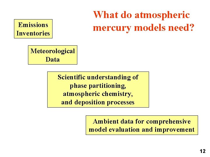
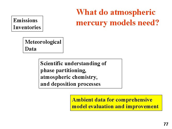
What do atmospheric mercury models need? Emissions Inventories Meteorological Data Scientific understanding of phase partitioning, atmospheric chemistry, and deposition processes Ambient data for comprehensive model evaluation and improvement 12

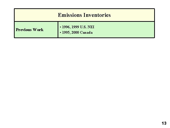
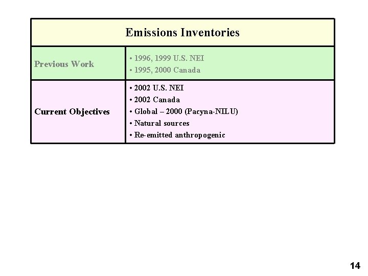
Emissions Inventories Previous Work • 1996, 1999 U. S. NEI • 1995, 2000 Canada 13

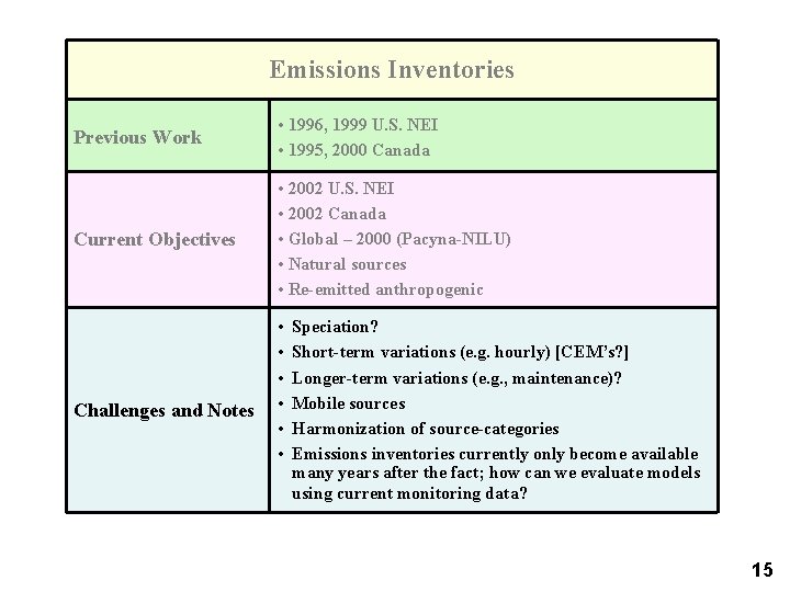
Emissions Inventories Previous Work • 1996, 1999 U. S. NEI • 1995, 2000 Canada Current Objectives • 2002 U. S. NEI • 2002 Canada • Global – 2000 (Pacyna-NILU) • Natural sources • Re-emitted anthropogenic 14

Emissions Inventories Previous Work • 1996, 1999 U. S. NEI • 1995, 2000 Canada Current Objectives • 2002 U. S. NEI • 2002 Canada • Global – 2000 (Pacyna-NILU) • Natural sources • Re-emitted anthropogenic Challenges and Notes • • • Speciation? Short-term variations (e. g. hourly) [CEM’s? ] Longer-term variations (e. g. , maintenance)? Mobile sources Harmonization of source-categories Emissions inventories currently only become available many years after the fact; how can we evaluate models using current monitoring data? 15

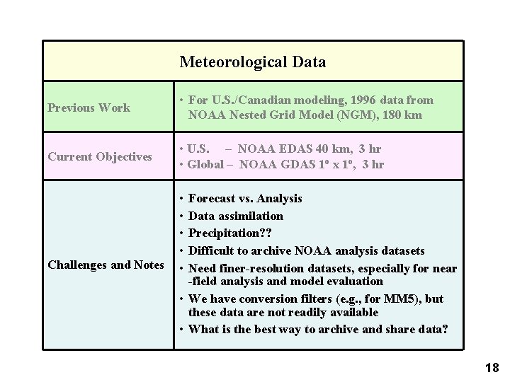
Meteorological Data Previous Work • For U. S. /Canadian modeling, 1996 data from NOAA Nested Grid Model (NGM), 180 km 16

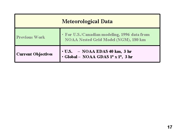
Meteorological Data Previous Work • For U. S. /Canadian modeling, 1996 data from NOAA Nested Grid Model (NGM), 180 km Current Objectives • U. S. – NOAA EDAS 40 km, 3 hr • Global – NOAA GDAS 1 o x 1 o, 3 hr 17

Meteorological Data Previous Work • For U. S. /Canadian modeling, 1996 data from NOAA Nested Grid Model (NGM), 180 km Current Objectives • U. S. – NOAA EDAS 40 km, 3 hr • Global – NOAA GDAS 1 o x 1 o, 3 hr Challenges and Notes • • • Forecast vs. Analysis Data assimilation Precipitation? ? Difficult to archive NOAA analysis datasets Need finer-resolution datasets, especially for near -field analysis and model evaluation • We have conversion filters (e. g. , for MM 5), but these data are not readily available • What is the best way to archive and share data? 18

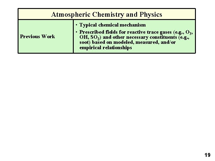
Atmospheric Chemistry and Physics Previous Work • Typical chemical mechanism • Prescribed fields for reactive trace gases (e. g. , O 3, OH, SO 2) and other necessary constituents (e. g. , soot) based on modeled, measured, and/or empirical relationships 19

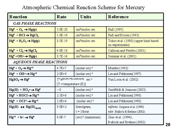
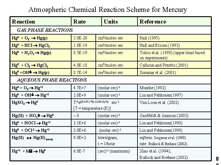
Atmospheric Chemical Reaction Scheme for Mercury Reaction Rate Units Reference Hg 0 + O 3 Hg(p) 3. 0 E-20 cm 3/molec-sec Hall (1995) Hg 0 + HCl Hg. Cl 2 1. 0 E-19 cm 3/molec-sec Hall and Bloom (1993) Hg 0 + H 2 O 2 Hg(p) 8. 5 E-19 cm 3/molec-sec Tokos et al. (1998) (upper limit based on experiments) Hg 0 + Cl 2 Hg. Cl 2 4. 0 E-18 cm 3/molec-sec Calhoun and Prestbo (2001) Hg 0 +OH • Hg(p) 8. 7 E-14 cm 3/molec-sec Sommar et al. (2001) GAS PHASE REACTIONS AQUEOUS PHASE REACTIONS Hg 0 + O 3 Hg+2 4. 7 E+7 (molar-sec)-1 Munthe (1992) Hg 0 + OH • Hg+2 2. 0 E+9 (molar-sec)-1 Lin and Pehkonen(1997) Hg. SO 3 Hg 0 T*e((31. 971*T)-12595. 0)/T) sec-1 [T = temperature (K)] Van Loon et al. (2002) Hg(II) + HO 2 • Hg 0 ~0 (molar-sec)-1 Gardfeldt & Jonnson (2003) Hg 0 + HOCl Hg+2 2. 1 E+6 (molar-sec)-1 Lin and Pehkonen(1998) Hg 0 + OCl-1 Hg+2 2. 0 E+6 (molar-sec)-1 Lin and Pehkonen(1998) Hg(II) (soot) 9. 0 E+2 liters/gram; t = 1/hour eqlbrm: Seigneur et al. (1998) rate: Bullock & Brehme (2002). Hg+2 + h< Hg 0 6. 0 E-7 (sec)-1 (maximum) Xiao et al. (1994); Bullock and Brehme (2002) 20

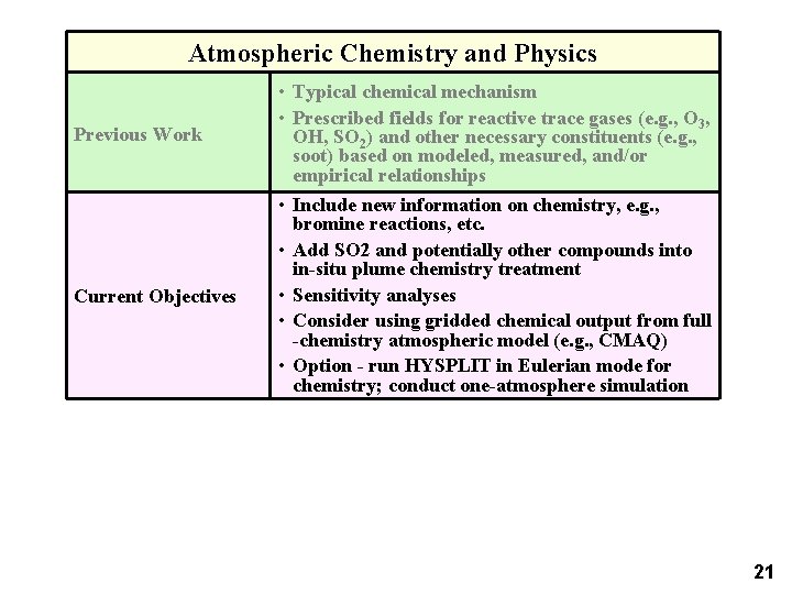
Atmospheric Chemistry and Physics Previous Work Current Objectives • Typical chemical mechanism • Prescribed fields for reactive trace gases (e. g. , O 3, OH, SO 2) and other necessary constituents (e. g. , soot) based on modeled, measured, and/or empirical relationships • Include new information on chemistry, e. g. , bromine reactions, etc. • Add SO 2 and potentially other compounds into in-situ plume chemistry treatment • Sensitivity analyses • Consider using gridded chemical output from full -chemistry atmospheric model (e. g. , CMAQ) • Option - run HYSPLIT in Eulerian mode for chemistry; conduct one-atmosphere simulation 21

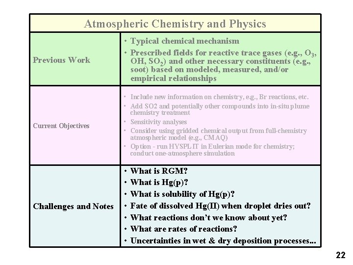
Atmospheric Chemistry and Physics Previous Work • Typical chemical mechanism • Prescribed fields for reactive trace gases (e. g. , O 3, OH, SO 2) and other necessary constituents (e. g. , soot) based on modeled, measured, and/or empirical relationships Current Objectives • Include new information on chemistry, e. g. , Br reactions, etc. • Add SO 2 and potentially other compounds into in-situ plume chemistry treatment • Sensitivity analyses • Consider using gridded chemical output from full-chemistry atmospheric model (e. g. , CMAQ) • Option - run HYSPLIT in Eulerian mode for chemistry; conduct one-atmosphere simulation Challenges and Notes • • What is RGM? What is Hg(p)? What is solubility of Hg(p)? Fate of dissolved Hg(II) when droplet dries out? What reactions don’t we know about yet? What are rates of reactions? Uncertainties in wet & dry deposition processes. . . 22

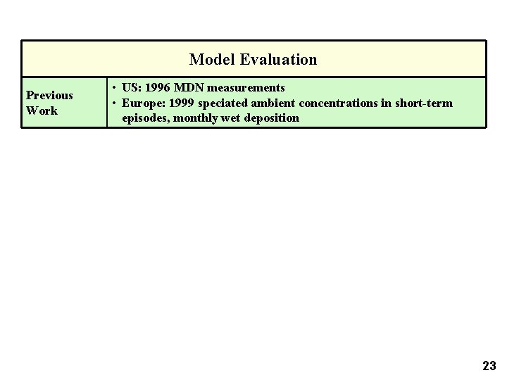
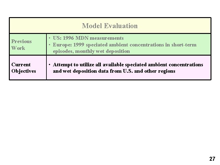
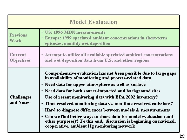
Model Evaluation Previous Work • US: 1996 MDN measurements • Europe: 1999 speciated ambient concentrations in short-term episodes, monthly wet deposition 23

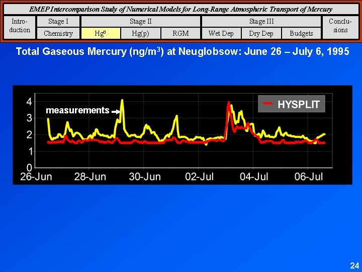
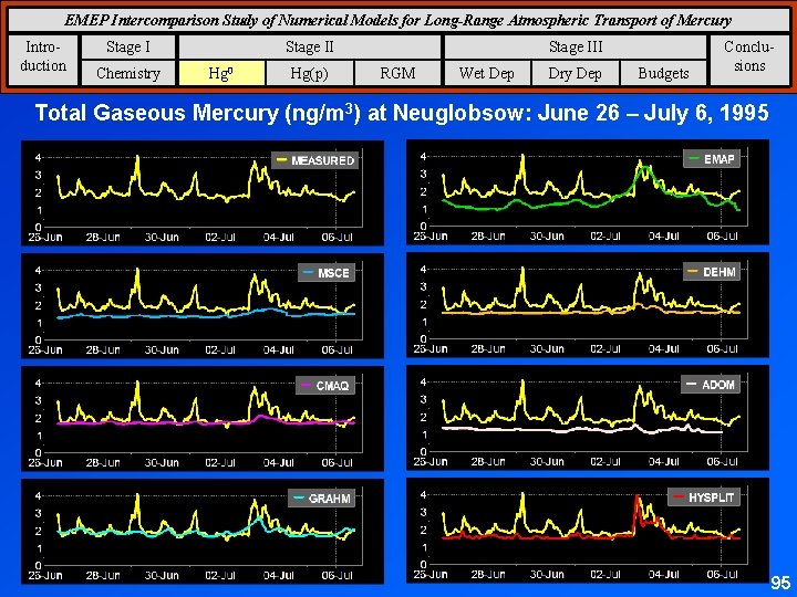
EMEP Intercomparison Study of Numerical Models for Long-Range Atmospheric Transport of Mercury Introduction Stage I Chemistry Stage II Hg 0 Hg(p) Stage III RGM Wet Dep Dry Dep Budgets Conclusions Total Gaseous Mercury (ng/m 3) at Neuglobsow: June 26 – July 6, 1995 measurements 24

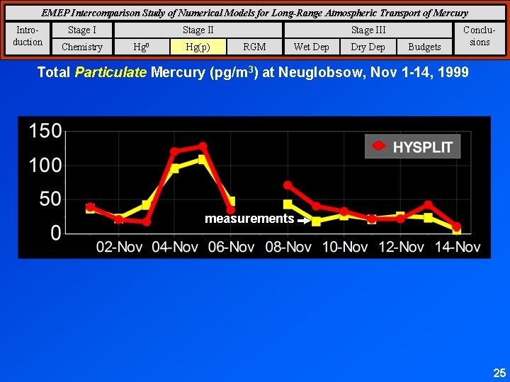
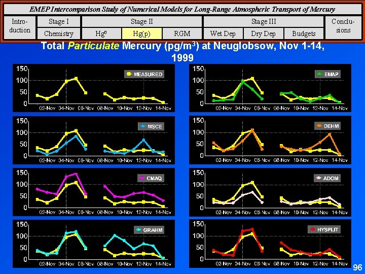
EMEP Intercomparison Study of Numerical Models for Long-Range Atmospheric Transport of Mercury Introduction Stage I Chemistry Stage II Hg 0 Hg(p) Stage III RGM Wet Dep Dry Dep Budgets Conclusions Total Particulate Mercury (pg/m 3) at Neuglobsow, Nov 1 -14, 1999 measurements 25

EMEP Intercomparison Study of Numerical Models for Long-Range Atmospheric Transport of Mercury Introduction Stage II Chemistry Hg 0 Hg(p) Stage III RGM Wet Dep Dry Dep Budgets Conclusions Reactive Gaseous Mercury at Neuglobsow, Nov 1 -14, 1999 26

Model Evaluation Previous Work • US: 1996 MDN measurements • Europe: 1999 speciated ambient concentrations in short-term episodes, monthly wet deposition Current Objectives • Attempt to utilize all available speciated ambient concentrations and wet deposition data from U. S. and other regions 27

Model Evaluation Previous Work • US: 1996 MDN measurements • Europe: 1999 speciated ambient concentrations in short-term episodes, monthly wet deposition Current Objectives • Attempt to utilize all available speciated ambient concentrations and wet deposition data from U. S. and other regions Challenges and Notes • Comprehensive evaluation has not been possible due to large gaps in availability of monitoring and process-related data • Need data for upper atmosphere as well as surface • Need data for both source-impacted and background sites • Use of recent monitoring data with EPA 2002 inventory? • Time-resolved monitoring data vs. non-time-resolved emissions? • Hard to diagnose differences between models & measurements • Can we find better ways to share data for model evaluation (and other purposes)? To this end, discussion is beginning on national, cooperative, ambient Hg monitoring network 28

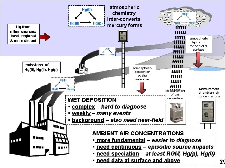
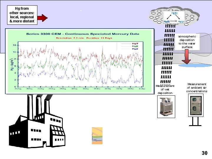
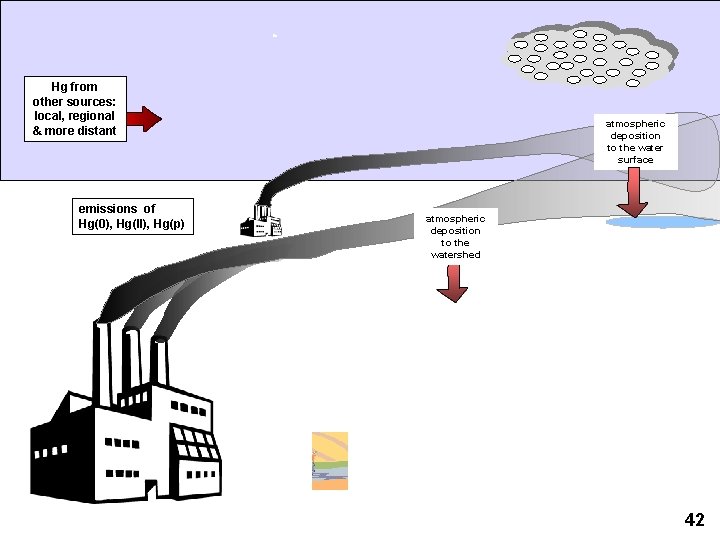
Hg(0) Hg from other sources: local, regional & more distant emissions of Hg(0), Hg(II), Hg(p) Hg(II) Hg(p) atmospheric chemistry inter-converts mercury forms atmospheric deposition to the water surface atmospheric deposition to the watershed WET DEPOSITION § complex – hard to diagnose § weekly – many events § background – also need near-field Measurement of wet deposition Measurement of ambient air concentrations AMBIENT AIR CONCENTRATIONS § more fundamental – easier to diagnose § need continuous – episodic source impacts § need speciation – at least RGM, Hg(p), Hg(0) § need data at surface and above 29

Hg from other sources: local, regional & more distant atmospheric deposition to the water surface atmospheric deposition to the watershed Measurement of wet deposition Measurement of ambient air concentrations 30

Source: Tekran Instruments Corporation 31

Example of results: Rock Creek Watershed 32

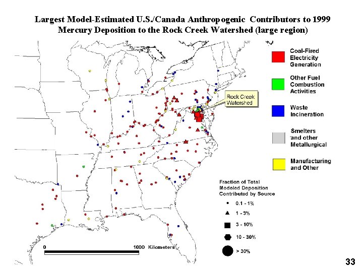
Largest Model-Estimated U. S. /Canada Anthropogenic Contributors to 1999 Mercury Deposition to the Rock Creek Watershed (large region) 33

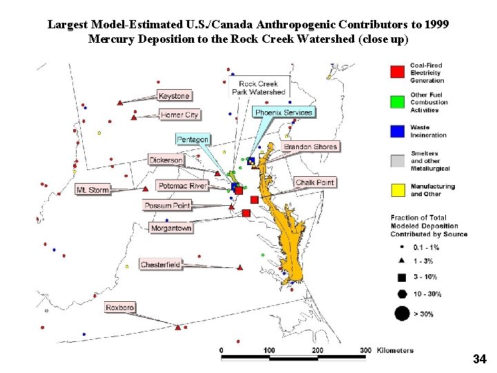
Largest Model-Estimated U. S. /Canada Anthropogenic Contributors to 1999 Mercury Deposition to the Rock Creek Watershed (close up) 34

Proportions of 1999 Model-Estimated Atmospheric Deposition to the Rock Creek Watershed from Different Anthropogenic U. S. /Canada Mercury Emissions Source Sectors 35

Top 25 Contributors to Hg Deposition to Rock Creek Watershed 36

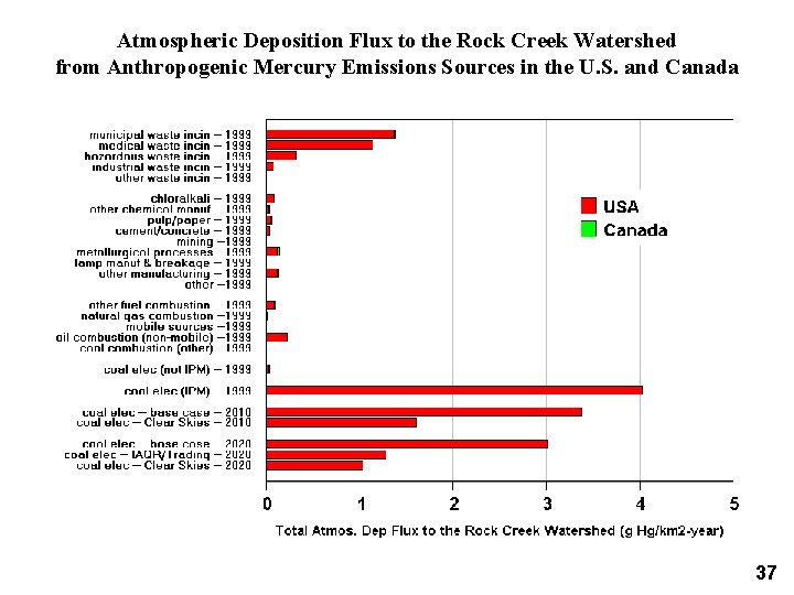
Atmospheric Deposition Flux to the Rock Creek Watershed from Anthropogenic Mercury Emissions Sources in the U. S. and Canada 37

Thanks! For more information on this research: http: //www. arl. noaa. gov/ss/transport/cohen. html 38

Extra Slides

Context

Hg from other sources: local, regional & more distant emissions of Hg(0), Hg(II), Hg(p) atmospheric deposition to the water surface atmospheric deposition to the watershed 42

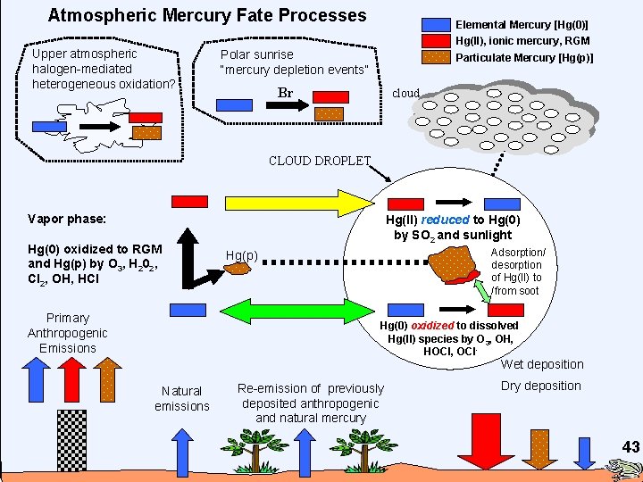
Atmospheric Mercury Fate Processes Upper atmospheric halogen-mediated heterogeneous oxidation? Elemental Mercury [Hg(0)] Hg(II), ionic mercury, RGM Polar sunrise “mercury depletion events” Particulate Mercury [Hg(p)] Br cloud CLOUD DROPLET Vapor phase: Hg(0) oxidized to RGM and Hg(p) by O 3, H 202, Cl 2, OH, HCl Primary Anthropogenic Emissions Hg(II) reduced to Hg(0) by SO 2 and sunlight Adsorption/ desorption of Hg(II) to /from soot Hg(p) Hg(0) oxidized to dissolved Hg(II) species by O 3, OH, HOCl, OCl- Wet deposition Natural emissions Re-emission of previously deposited anthropogenic and natural mercury Dry deposition 43

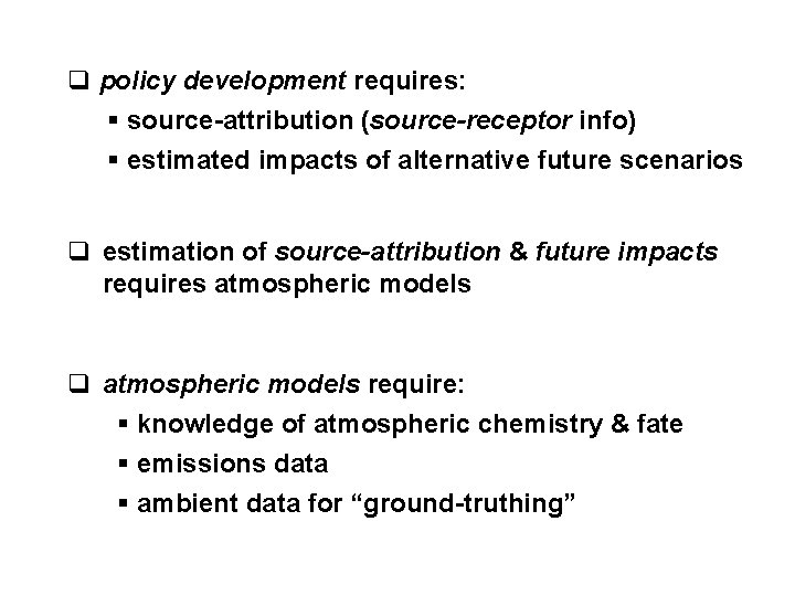
q policy development requires: § source-attribution (source-receptor info) § estimated impacts of alternative future scenarios q estimation of source-attribution & future impacts requires atmospheric models q atmospheric models require: § knowledge of atmospheric chemistry & fate § emissions data § ambient data for “ground-truthing”

methodology

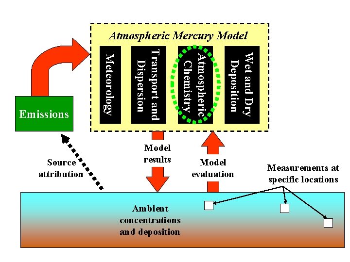
Atmospheric Mercury Model Ambient concentrations and deposition Wet and Dry Deposition Model results Atmospheric Chemistry Transport and Dispersion Source attribution Meteorology Emissions Model evaluation Measurements at specific locations

Some Current Atmospheric Chemistry Challenges q Plume chemistry, e. g. , rapid reduction of RGM to elemental mercury? Ø If significant reduction of RGM to Hg(0) is occurring in power-plant plumes, then much less local/regional deposition 47

RGM reduction in power-plant plumes? q If significant reduction of RGM to Hg(0) is occurring in power-plant plumes, then much less local/regional deposition q No known chemical reaction is capable of causing significant reduction of RGM in plumes – e. g. measured rates of SO 2 reduction can’t explain some of the claimed reduction rates q Very hard to measure q Aircraft q Static Plume Dilution Chambers (SPDC) q Ground-based measurements 48

RGM reduction in power-plant plumes? q Most current state-of-the-science models do not include processes that lead to significant reduction in plumes q Recent measurement results show less reduction q Significant uncertainties – e. g. , mass balance errors comparable to measured effects… q Current status – inconclusive… but weight of evidence suggest that while some reduction may be occurring, it may be only a relatively small amount q Recent measurements at Steubenville, OH appear to show strong local mercury deposition from coal-fired power plant emissions. 49

Some Current Atmospheric Chemistry Challenges q Plume chemistry, e. g. , rapid reduction of RGM to elemental mercury? q Boundary conditions for regional models? 50

Some Current Atmospheric Chemistry Challenges q Plume chemistry, e. g. , rapid reduction of RGM to elemental mercury? q Boundary conditions for regional models? q Oxidation of elemental mercury by O 3 and OH • may be over-represented, leading to overestimation of the contribution of global sources to regional deposition Calvert, J. , and S. Lindberg (2005). Mechanisms of mercury removal by O 3 and OH in the atmosphere. Atmospheric Environment 39: 3355 -3367. 51

Some Current Atmospheric Chemistry Challenges q Plume chemistry, e. g. , rapid reduction of RGM to elemental mercury? q Boundary conditions for regional models? q Oxidation of elemental mercury by O 3 and OH • may be over-represented, leading to overestimation of the contribution of global sources to regional deposition Calvert, J. , and S. Lindberg (2005). Mechanisms of mercury removal by O 3 and OH in the atmosphere. Atmospheric Environment 39: 3355 -3367. q Atmospheric methyl-mercury: significance? sources? transport? chemistry? deposition? e. g. , Hall et al. (2005). Methyl and total mercury in precipitation in the Great Lakes region. Atmospheric Environment 39: 7557 -7569. 52

Some Current Atmospheric Chemistry Challenges q Plume chemistry, e. g. , rapid reduction of RGM to elemental mercury? q Boundary conditions for regional models? q Oxidation of elemental mercury by O 3 and OH • may be over-represented, leading to overestimation of the contribution of global sources to regional deposition Calvert, J. , and S. Lindberg (2005). Mechanisms of mercury removal by O 3 and OH in the atmosphere. Atmospheric Environment 39: 3355 -3367. q Atmospheric methyl-mercury: significance? sources? transport? chemistry? deposition? e. g. , Hall et al. (2005). Methyl and total mercury in precipitation in the Great Lakes region. Atmospheric Environment 39: 7557 -7569. q Source-Receptor answers influenced by above factors 53

emissions

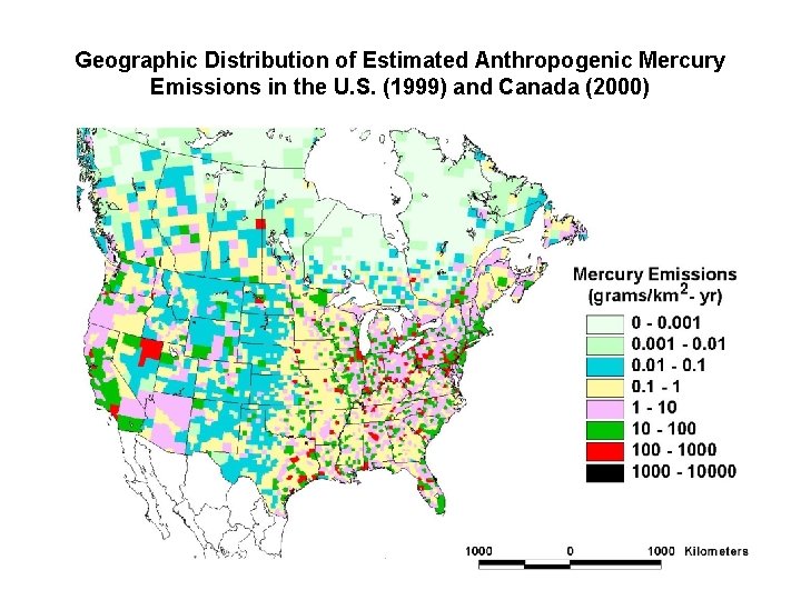
Geographic Distribution of Estimated Anthropogenic Mercury Emissions in the U. S. (1999) and Canada (2000)

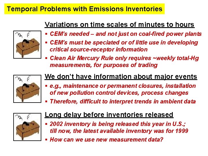
Temporal Problems with Emissions Inventories Variations on time scales of minutes to hours § CEM’s needed – and not just on coal-fired power plants § CEM’s must be speciated or of little use in developing critical source-receptor information § Clean Air Mercury Rule only requires ~weekly total-Hg measurements, for purposes of trading We don’t have information about major events § e. g. , maintenance or permanent closures, installation of new pollution control devices, process changes § Therefore, difficult to interpret trends in ambient data Long delay before inventories released § 2002 inventory is being released this year in U. S. ; till now, the latest available inventory was for 1999 § How can we use new measurement data?

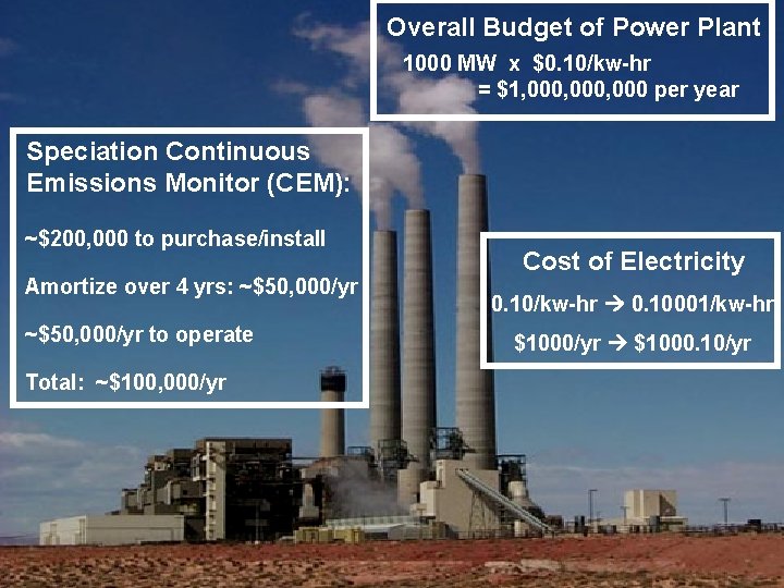
Overall Budget of Power Plant 1000 MW x $0. 10/kw-hr = $1, 000, 000 per year Speciation Continuous Emissions Monitor (CEM): ~$200, 000 to purchase/install Amortize over 4 yrs: ~$50, 000/yr to operate Total: ~$100, 000/yr Cost of Electricity 0. 10/kw-hr 0. 10001/kw-hr $1000/yr $1000. 10/yr

illustrative model results

Why are emissions speciation data - and potential plume transformations -- critical? Logarithmic NOTE: distance results averaged over all directions – Some directions will have higher fluxes, some will have lower 59

sourcereceptor results

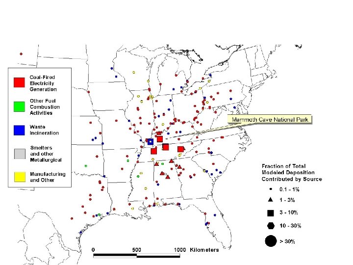
Figure __. Hg Deposition From U. S. Coal-Fired Power Plants in 1999

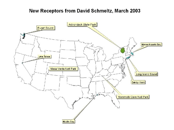
Results for Mammoth Cave National Park

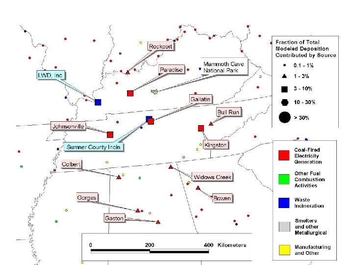
Top 25 Contributors to Hg Deposition to Mammoth Cave National Park

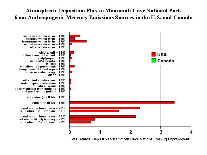
Atmospheric Deposition Flux to Mammoth Cave National Park from Anthropogenic Mercury Emissions Sources in the U. S. and Canada

Results for Chesapeake Bay

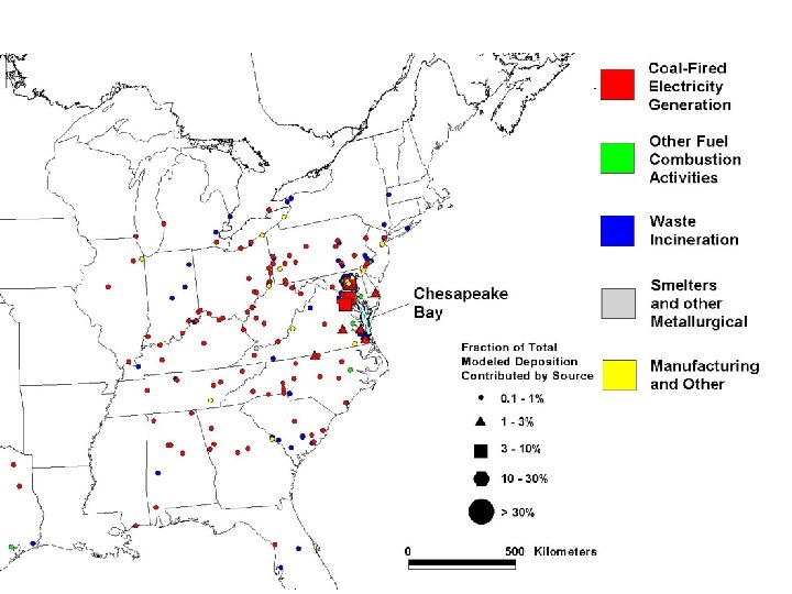
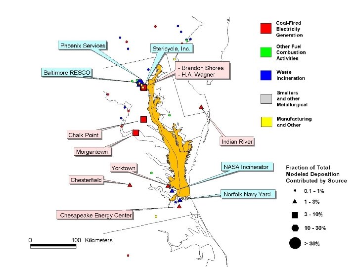
Top 25 Contributors to 1999 Hg Deposition Directly to the Chesapeake Bay

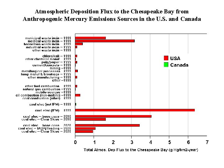
Atmospheric Deposition Flux to the Chesapeake Bay from Anthropogenic Mercury Emissions Sources in the U. S. and Canada

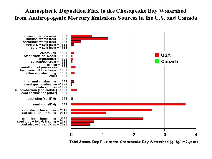
Atmospheric Deposition Flux to the Chesapeake Bay Watershed from Anthropogenic Mercury Emissions Sources in the U. S. and Canada

model evaluation

Emissions Inventories What do atmospheric mercury models need? Meteorological Data Scientific understanding of phase partitioning, atmospheric chemistry, and deposition processes Ambient data for comprehensive model evaluation and improvement 77

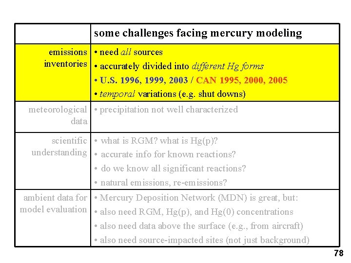
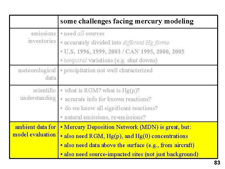
some challenges facing mercury modeling emissions • need all sources inventories • accurately divided into different Hg forms • U. S. 1996, 1999, 2003 / CAN 1995, 2000, 2005 • temporal variations (e. g. shut downs) meteorological • precipitation not well characterized data scientific • what is RGM? what is Hg(p)? understanding • accurate info for known reactions? • do we know all significant reactions? • natural emissions, re-emissions? ambient data for • Mercury Deposition Network (MDN) is great, but: model evaluation • also need RGM, Hg(p), and Hg(0) concentrations • also need data above the surface (e. g. , from aircraft) • also need source-impacted sites (not just background) 78

Why is emissions speciation information critical? Logarithmic Hypothesized rapid reduction of Hg(II) in plumes? If true, then dramatic impact on modeling results… 79

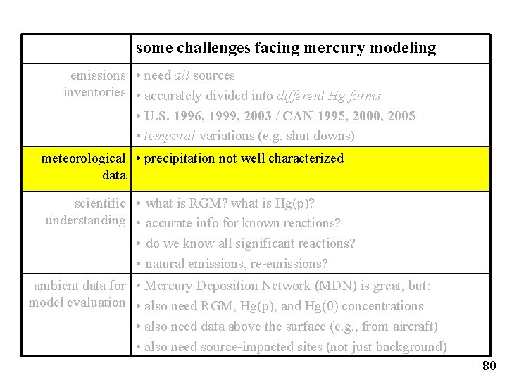
some challenges facing mercury modeling emissions • need all sources inventories • accurately divided into different Hg forms • U. S. 1996, 1999, 2003 / CAN 1995, 2000, 2005 • temporal variations (e. g. shut downs) meteorological • precipitation not well characterized data scientific • what is RGM? what is Hg(p)? understanding • accurate info for known reactions? • do we know all significant reactions? • natural emissions, re-emissions? ambient data for • Mercury Deposition Network (MDN) is great, but: model evaluation • also need RGM, Hg(p), and Hg(0) concentrations • also need data above the surface (e. g. , from aircraft) • also need source-impacted sites (not just background) 80

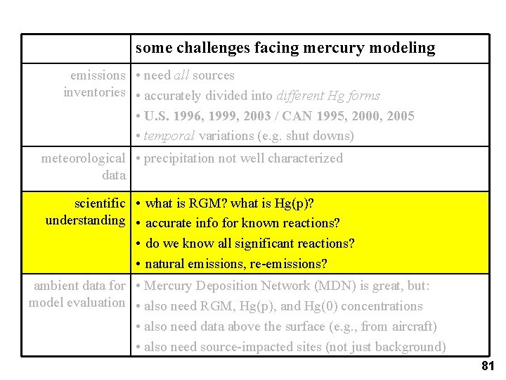
some challenges facing mercury modeling emissions • need all sources inventories • accurately divided into different Hg forms • U. S. 1996, 1999, 2003 / CAN 1995, 2000, 2005 • temporal variations (e. g. shut downs) meteorological • precipitation not well characterized data scientific • what is RGM? what is Hg(p)? understanding • accurate info for known reactions? • do we know all significant reactions? • natural emissions, re-emissions? ambient data for • Mercury Deposition Network (MDN) is great, but: model evaluation • also need RGM, Hg(p), and Hg(0) concentrations • also need data above the surface (e. g. , from aircraft) • also need source-impacted sites (not just background) 81

Atmospheric Chemical Reaction Scheme for Mercury Reaction Rate Units Reference Hg 0 + O 3 Hg(p) 3. 0 E-20 cm 3/molec-sec Hall (1995) Hg 0 + HCl Hg. Cl 2 1. 0 E-19 cm 3/molec-sec Hall and Bloom (1993) Hg 0 + H 2 O 2 Hg(p) 8. 5 E-19 cm 3/molec-sec Tokos et al. (1998) (upper limit based on experiments) Hg 0 + Cl 2 Hg. Cl 2 4. 0 E-18 cm 3/molec-sec Calhoun and Prestbo (2001) Hg 0 +OHC Hg(p) 8. 7 E-14 cm 3/molec-sec Sommar et al. (2001) GAS PHASE REACTIONS AQUEOUS PHASE REACTIONS Hg 0 + O 3 Hg+2 4. 7 E+7 (molar-sec)-1 Munthe (1992) Hg 0 + OHC Hg+2 2. 0 E+9 (molar-sec)-1 Lin and Pehkonen(1997) Hg. SO 3 Hg 0 T*e((31. 971*T)-12595. 0)/T) sec-1 [T = temperature (K)] Van Loon et al. (2002) Hg(II) + HO 2 C Hg 0 ~0 (molar-sec)-1 Gardfeldt & Jonnson (2003) Hg 0 + HOCl Hg+2 2. 1 E+6 (molar-sec)-1 Lin and Pehkonen(1998) Hg 0 + OCl-1 Hg+2 2. 0 E+6 (molar-sec)-1 Lin and Pehkonen(1998) Hg(II) (soot) 9. 0 E+2 liters/gram; t = 1/hour eqlbrm: Seigneur et al. (1998) rate: Bullock & Brehme (2002). Hg+2 + h< Hg 0 6. 0 E-7 (sec)-1 (maximum) Xiao et al. (1994); Bullock and Brehme (2002) 8

some challenges facing mercury modeling emissions • need all sources inventories • accurately divided into different Hg forms • U. S. 1996, 1999, 2003 / CAN 1995, 2000, 2005 • temporal variations (e. g. shut downs) meteorological • precipitation not well characterized data scientific • what is RGM? what is Hg(p)? understanding • accurate info for known reactions? • do we know all significant reactions? • natural emissions, re-emissions? ambient data for • Mercury Deposition Network (MDN) is great, but: model evaluation • also need RGM, Hg(p), and Hg(0) concentrations • also need data above the surface (e. g. , from aircraft) • also need source-impacted sites (not just background) 83

Some Additional Measurement Issues (from a modeler’s perspective) • Data availability • Simple vs. Complex Measurements

Some Additional Measurement Issues (from a modeler’s perspective) • Data availability • Simple vs. Complex Measurements

Data availability A major impediment to evaluating and improving atmospheric Hg models has been the lack of speciated Hg air concentration data There have been very few measurements to date, and these data are rarely made available in a practical way (timely, complete, etc. ) The data being collected at Piney Reservoir could be extremely helpful!

Some Additional Measurement Issues (from a modeler’s perspective) • Data availability • Simple vs. Complex Measurements

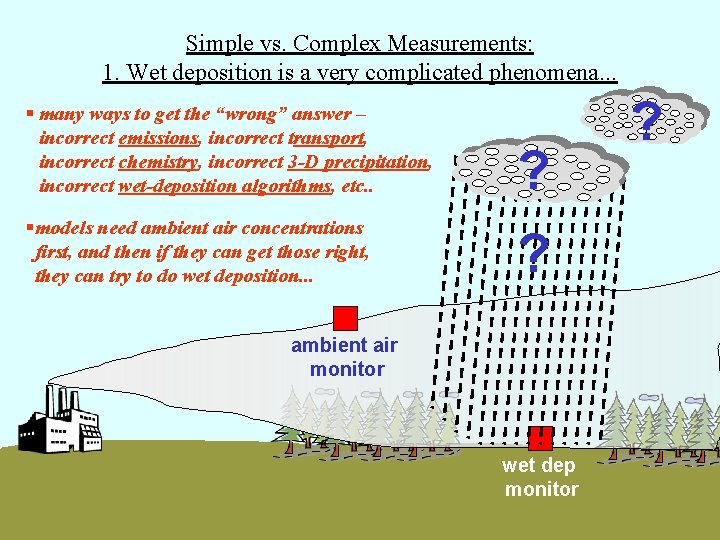
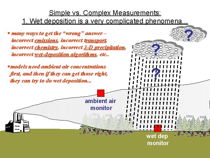
Simple vs. Complex Measurements: 1. Wet deposition is a very complicated phenomena. . . § many ways to get the “wrong” answer – incorrect emissions, incorrect transport, incorrect chemistry, incorrect 3 -D precipitation, incorrect wet-deposition algorithms, etc. . ? §models need ambient air concentrations first, and then if they can get those right, they can try to do wet deposition. . . ? ambient air monitor wet dep monitor ?

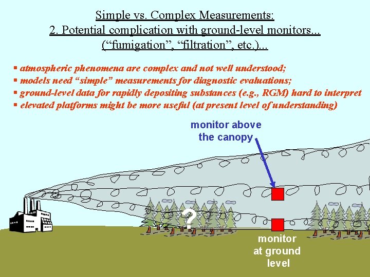
Simple vs. Complex Measurements: 2. Potential complication with ground-level monitors. . . (“fumigation”, “filtration”, etc. ). . . § atmospheric phenomena are complex and not well understood; § models need “simple” measurements for diagnostic evaluations; § ground-level data for rapidly depositing substances (e. g. , RGM) hard to interpret § elevated platforms might be more useful (at present level of understanding) monitor above the canopy ? monitor at ground level

Simple vs. Complex measurements - 3. Urban areas: a. Emissions inventory poorly known b. Meteorology very complex (flow around buildings) c. So, measurements in urban areas not particularly useful for current large-scale model evaluations

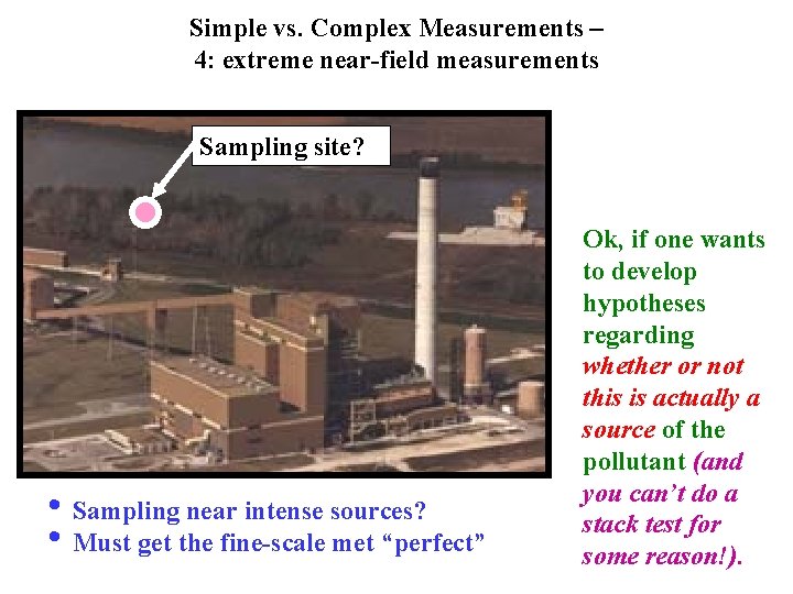
Simple vs. Complex Measurements – 4: extreme near-field measurements Sampling site? • Sampling near intense sources? • Must get the fine-scale met “perfect” Ok, if one wants to develop hypotheses regarding whether or not this is actually a source of the pollutant (and you can’t do a stack test for some reason!).

Complex vs. Simple Measurements – 5: Need some source impacted measurements • Major questions regarding plume chemistry and near-field impacts (are there “hot spots”? ) • Most monitoring sites are designed to be “regional background” sites (e. g. , most Mercury Deposition Network sites). • We need some source-impacted sites as well to help resolve near-field questions • But not too close – maybe 20 -30 km is ideal (? )

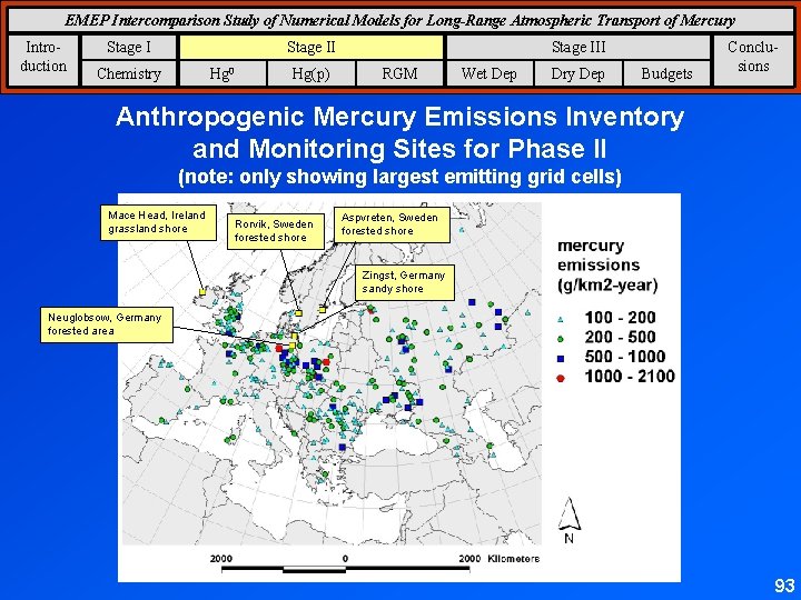
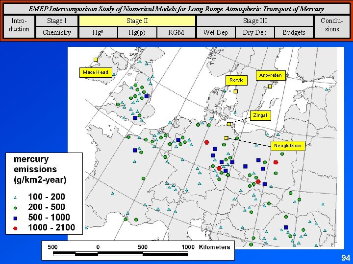
EMEP Intercomparison Study of Numerical Models for Long-Range Atmospheric Transport of Mercury Introduction Stage II Chemistry Hg 0 Hg(p) Stage III RGM Wet Dep Dry Dep Budgets Conclusions Anthropogenic Mercury Emissions Inventory and Monitoring Sites for Phase II (note: only showing largest emitting grid cells) Mace Head, Ireland grassland shore Rorvik, Sweden forested shore Aspvreten, Sweden forested shore Zingst, Germany sandy shore Neuglobsow, Germany forested area 93

EMEP Intercomparison Study of Numerical Models for Long-Range Atmospheric Transport of Mercury Introduction Stage I Chemistry Stage II Hg 0 Hg(p) Stage III RGM Wet Dep Dry Dep Mace Head Rorvik Budgets Conclusions Aspvreten Zingst Neuglobsow 94

EMEP Intercomparison Study of Numerical Models for Long-Range Atmospheric Transport of Mercury Introduction Stage I Chemistry Stage II Hg 0 Hg(p) Stage III RGM Wet Dep Dry Dep Budgets Conclusions Total Gaseous Mercury (ng/m 3) at Neuglobsow: June 26 – July 6, 1995 95

EMEP Intercomparison Study of Numerical Models for Long-Range Atmospheric Transport of Mercury Introduction Stage I Chemistry Stage II Hg 0 Hg(p) Stage III RGM Wet Dep Dry Dep Budgets Conclusions Total Particulate Mercury (pg/m 3) at Neuglobsow, Nov 1 -14, 1999 96

Simple vs. Complex Measurements: 1. Wet deposition is a very complicated phenomena. . . § many ways to get the “wrong” answer – incorrect emissions, incorrect transport, incorrect chemistry, incorrect 3 -D precipitation, incorrect wet-deposition algorithms, etc. . ? §models need ambient air concentrations first, and then if they can get those right, they can try to do wet deposition. . . ? ambient air monitor wet dep monitor ?

speciated ambient concentration data is scarce § few measurement sites at ground level § very few measurements aloft therefore, atmospheric mercury models have not really been comprehensively evaluated yet § we don’t really know how good or bad they are collaboration between measurement and modeling community is key § measurers need modelers to help interpret data § modelers need measurements to evaluate models

model intercomparison

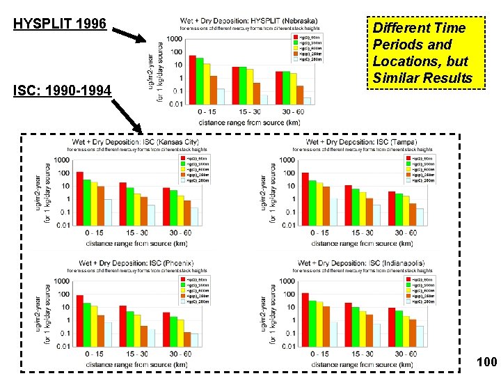
HYSPLIT 1996 ISC: 1990 -1994 Different Time Periods and Locations, but Similar Results 100

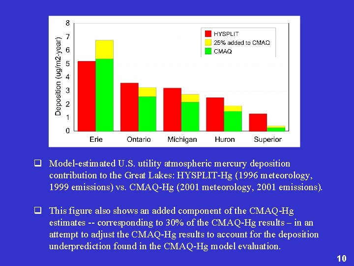
Model-estimated U. S. utility atmospheric mercury deposition contribution to the Great Lakes: HYSPLIT-Hg (1996 meteorology, 1999 emissions) vs. CMAQ-HG (2001 meteorology, 2001 emissions). 10

q Model-estimated U. S. utility atmospheric mercury deposition contribution to the Great Lakes: HYSPLIT-Hg (1996 meteorology, 1999 emissions) vs. CMAQ-Hg (2001 meteorology, 2001 emissions). q This figure also shows an added component of the CMAQ-Hg estimates -- corresponding to 30% of the CMAQ-Hg results – in an attempt to adjust the CMAQ-Hg results to account for the deposition underprediction found in the CMAQ-Hg model evaluation. 10

MANY THANKS TO: q Gary Foley, J. David Mobley, Elsie Sunderland, Chris Knightes (EPA); Panos Georgopolous and Sheng-Wei Wang (EOSHI Rutgers Univ); John Mc. Donald (IJC): collaboration on multimedia Hg modeling q David Schmeltz, Gary Lear, John Schakenbach, Scott Hedges, Rey Forte (EPA): collaboration on Hg models and /measurements, including new EPA-NOAA Hg monitoring site at Beltsville, MD. q David Ruple, Mark Woodrey (Grand Bay NERR), Susan White , Gary Matlock, Russell Callender, Jawed Hameedi (NOAA), and Durwin Carter (U. S. Fish and Wildlife Service): collaboration at NOAA Grand Bay NERR atmospheric monitoring site q Anne Pope and colleagues (EPA): U. S. mercury emissions inventory q David Niemi, Dominique Ratte, Marc Deslauriers (Environment Canada): mercury emissions inventory data Canadian q Mark Castro (Univ. Md, Frostburg), Fabien Laurier (Univ Md Ches Biol Lab), Rob Mason (Univ CT), Laurier Poissant (Envr Can): ambient Hg data for model evaluation q Roland Draxler, Glenn Rolph, Rick Artz (NOAA): HYSPLIT model and met data q Steve Brooks, Winston Luke, Paul Kelley (NOAA) : ambient Hg data