Advanced Physical Chemistry G H CHEN Department of

Advanced Physical Chemistry G. H. CHEN Department of Chemistry University of Hong Kong

Quantum Chemistry G. H. Chen Department of Chemistry University of Hong Kong

Emphasis Hartree-Fock method Concepts Hands-on experience Text Book “Quantum Chemistry”, 4 th Ed. Ira N. Levine http: //yangtze. hku. hk/lecture/chem 3504 -3. ppt

Beginning of Computational Chemistry In 1929, Dirac declared, “The underlying physical laws necessary for the mathematical theory of. . . the whole of chemistry are thus completely know, and the difficulty is only that the exact application of these laws leads to equations much too complicated to be soluble. ” Dirac

Quantum Chemistry Methods • Ab initio molecular orbital methods • Semiempirical molecular orbital methods • Density functional method

SchrÖdinger Equation H =E Wavefunction Hamiltonian H = (-h 2/2 m ) 2 - (h 2/2 me) i i 2 + Z Z e 2/r - i Z e 2/ri + i j e 2/rij Energy Contents 1. Variation Method 2. Hartree-Fock Self-Consistent Field Method

The Variation Method The variation theorem Consider a system whose Hamiltonian operator H is time independent and whose lowest-energy eigenvalue is E 1. If is any normalized, wellbehaved function that satisfies the boundary conditions of the problem, then * H dt > E 1

Proof: Expand in the basis set { k} where then = k k k { k} are coefficients H k = Ek k * H dt = k j k* j Ej kj 2 E > E | |2 = E = | | k k k 1 k k 1 Since is normalized, * dt = k | k|2 = 1

i. : trial function is used to evaluate the upper limit of ground state energy E 1 ii. = ground state wave function, * H d = E 1 iii. optimize paramemters in by minimizing * H d / * d

Application to a particle in a box of infinite depth 0 l Requirements for the trial wave function: i. zero at boundary; ii. smoothness a maximum in the center. Trial wave function: = x (l - x)

* H dx = -(h 2/8 2 m) (lx-x 2) d 2(lx-x 2)/dx 2 dx = h 2/(4 2 m) (x 2 - lx) dx = h 2 l 3/(24 2 m) * dx = x 2 (l-x)2 dx = l 5/30 E = 5 h 2/(4 2 l 2 m) h 2/(8 ml 2) = E 1

Variational Method (1) Construct a wave function (c 1, c 2, , cm) (2) Calculate the energy of : E E (c 1, c 2, , cm) (3) Choose {cj*} (i=1, 2, , m) so that E is minimum

Example: one-dimensional harmonic oscillator Potential: V(x) = (1/2) kx 2 = (1/2) m 2 x 2 = 2 2 m 2 x 2 Trial wave function for the ground state: (x) = exp(-cx 2) * H dx = -(h 2/8 2 m) exp(-cx 2) d 2[exp(-cx 2)]/dx 2 dx + 2 2 m 2 x 2 exp(-2 cx 2) dx = (h 2/4 2 m) ( c/8)1/2 + 2 m 2 ( /8 c 3)1/2 * dx = exp(-2 cx 2) dx = ( /2)1/2 c-1/2 E = W = (h 2/8 2 m)c + ( 2/2)m 2/c

To minimize W, 0 = d. W/dc = h 2/8 2 m - ( 2/2)m 2 c-2 c = 2 2 m/h W = (1/2) h

Extension of Variation Method . . . E 3 3 E 2 2 E 1 1 For a wave function which is orthogonal to the ground state wave function 1, i. e. dt * 1 = 0 E = dt *H / dt * > E 2 the first excited state energy

The trial wave function : dt * 1 = 0 = k=1 ak k dt * 1 = |a 1|2 = 0 E = dt *H / dt * = k=2|ak|2 Ek / k=2|ak|2 > k=2|ak|2 E 2 / k=2|ak|2 = E 2

Application to H 2+ e + 1 2 = c + c 1 1 2 2 W = *H dt / * dt = (c 12 H 11 + 2 c 1 c 2 H 12 + c 22 H 22 ) / (c 12 + 2 c 1 c 2 S + c 22 ) W (c 12 + 2 c 1 c 2 S + c 22) = c 12 H 11 + 2 c 1 c 2 H 12 + c 22 H 22

Partial derivative with respect to c 1 ( W/ c 1 = 0) : W (c 1 + S c 2) = c 1 H 11 + c 2 H 12 Partial derivative with respect to c 2 ( W/ c 2 = 0) : W (S c 1 + c 2) = c 1 H 12 + c 2 H 22 (H 11 - W) c 1 + (H 12 - S W) c 2 = 0 (H 12 - S W) c 1 + (H 22 - W) c 2 = 0

To have nontrivial solution: H 11 - W H 12 - S W = 0 H 12 - S W H 22 - W For H 2+, H 11 = H 22; H 12 < 0. Ground State: Eg = W 1 = (H 11+H 12) / (1+S) 1 = ( 1+ 2) / 2(1+S)1/2 bonding orbital Excited State: Ee = W 2 = (H 11 -H 12) / (1 -S) 2 = ( 1 - 2) / 2(1 -S)1/2 Anti-bonding orbital

Results: De = 1. 76 e. V, Re = 1. 32 A Exact: De = 2. 79 e. V, Re = 1. 06 A 1 e. V = 23. 0605 kcal / mol

Further Improvements Optimization of 1 s orbitals H He+ -1/2 exp(-r) 23/2 -1/2 exp(-2 r) Trial wave function: k 3/2 -1/2 exp(-kr) Eg = W 1(k, R) at each R, choose k so that W 1/ k = 0 Results: De = 2. 36 e. V, Re = 1. 06 A Inclusion of other atomic orbitals 1 s 2 p Resutls: De = 2. 73 e. V, Re = 1. 06 A

Linear Equations 1. two linear equations for two unknown, x 1 and x 2 a 11 x 1 + a 12 x 2 = b 1 a 21 x 1 + a 22 x 2 = b 2 (a 11 a 22 -a 12 a 21) x 1 = b 1 a 22 -b 2 a 12 (a 11 a 22 -a 12 a 21) x 2 = b 2 a 11 -b 1 a 21

Introducing determinant: a 11 a 12 = a 11 a 22 -a 12 a 21 a 22 a 11 a 12 b 1 a 12 x 1 = a 21 a 22 b 2 a 22 a 11 a 12 a 11 b 1 x 2 = a 21 a 22 a 21 b 2

Our case: b 1 = b 2 = 0, homogeneous 1. trivial solution: x 1 = x 2 = 0 2. nontrivial solution: a 11 a 12 = 0 a 21 a 22 n linear equations for n unknown variables a 11 x 1 + a 12 x 2 +. . . + a 1 nxn= b 1 a 21 x 1 + a 22 x 2 +. . . + a 2 nxn= b 2. . . an 1 x 1 + an 2 x 2 +. . . + annxn= bn

a 11 a 21 det(aij) xk= . an 1 where, a 11 a 21 det(aij) = . an 1 a 12 a 22 . an 2 . . . a 1, k-1 b 1 a 1, k+1. . . a 1 n . . . a 2, k-1 b 2 a 2, k+1. . . a 2 n . . . . . . an, k-1 b 2 an, k+1. . . ann a 12 a 22 . an 2 . . . a 1 n a 2 n . ann

inhomogeneous case: bk = 0 for at least one k xk = a 11 a 21 . an 1 a 12 a 22 . an 2 . . . a 1, k-1 a 2, k-1 . an, k-1 det(aij) b 1 b 2 a 1, k+1. . . a 2, k+1. . an, k+1. . . a 1 n a 2 n . ann

homogeneous case: bk = 0, k = 1, 2, . . . , n (a) travial case: xk = 0, k = 1, 2, . . . , n (b) nontravial case: det(aij) = 0 For a n-th order determinant, n det(aij) = alk Clk l=1 where, Clk is called cofactor

Trial wave function is a variation function which is a combination of n linear independent functions { f 1 , f 2 , . . . fn}, = c 1 f 1 + c 2 f 2 +. . . + cnfn n [( Hik - Sik. W ) ck ] = 0 i=1, 2, . . . , n k=1 Sik dt fi fk Hik dt fi H fk W dt H / dt

Linear variational theorem (i) W 1 W 2 . . . Wn are n roots of Eq. (1), (ii) E 1 E 2 . . . En+1 . . . are energies of eigenstates; then, W 1 E 1, W 2 E 2, . . . , Wn En

Molecular Orbital (MO): = c 1 1 + c 2 2 ( H 11 - W ) c 1 + ( H 12 - SW ) c 2 = 0 S 11=1 ( H 21 - SW ) c 1 + ( H 22 - W ) c 2 = 0 S 22=1 Generally : i a set of atomic orbitals, basis set LCAO-MO = c 1 1 + c 2 2 +. . . + cn n linear combination of atomic orbitals n ( Hik - Sik. W ) ck = 0 i = 1, 2, . . . , n k=1 Hik dt i* H k Sik dt i* k Skk = 1

The Born-Oppenheimer Approximation Hamiltonian H = (-h 2/2 m ) 2 - (h 2/2 me) i i 2 + Z Z e 2/r - i Z e 2/ri + i j e 2/rij H (ri; r ) = E (ri; r )

The Born-Oppenheimer Approximation: (1) (ri; r ) = el(ri; r ) N(r ) (2) Hel(r )= - (h 2/2 me) i i 2 - i Z e 2/ri + i j e 2/rij VNN = Z Z e 2/r Hel(r ) el(ri; r ) = Eel(r ) el(ri; r ) (3) HN = (-h 2/2 m ) 2 + U(r ) = Eel(r ) + VNN HN(r ) = E N(r )

Assignment Calculate the ground state energy and bond length of H 2 using the Hyper. Chem with the 6 -31 G (Hint: Born-Oppenheimer Approximation)

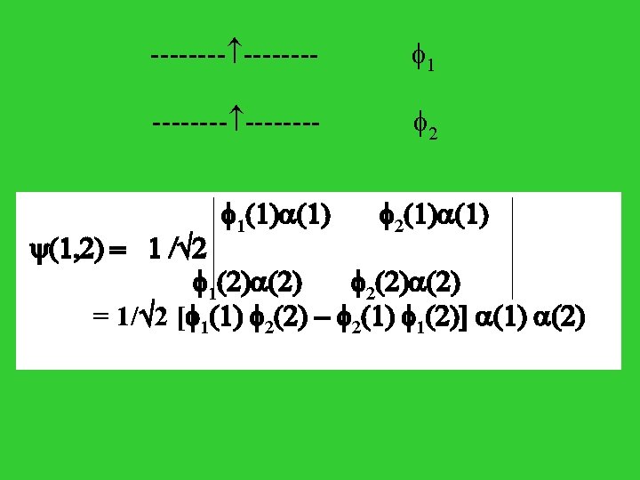
Hydrogen Molecule H 2 e + e The Pauli principle two electrons cannot be in the same state.

Wave function: (1, 2) = ja(1)jb(2) + c 1 ja(2)jb(1) (2, 1) = ja(2)jb(1) + c 1 ja(1)jb(2) Since two wave functions that correspond to the same state can differ at most by a constant factor (1, 2) = c 2 (2, 1) ja(1)jb(2) + c 1 ja(2)jb(1) =c 2 ja(2)jb(1) +c 2 c 1 ja(1)jb(2) c 1 = c 2 c 1 = 1 Therefore: c 1 = c 2 = 1 According to the Pauli principle, c 1 = c 2 =- 1

The Pauli principle (different version) the wave function of a system of electrons must be antisymmetric with respect to interchanging of any two electrons. Wave function of H 2 : Slater Determinant (1, 2) = 1/ 2! [ (1) (2) - (2) (1)] (1) = 1/ 2! (1) (2) (2)

Energy: E E =2 d 1 *(1) (Te+Ve. N) (1) + VNN + d 1 d 2 | 2(1)| e 2/r 12 | 2(2)| = i=1, 2 fii + J 12 + VNN To minimize E under the constraint dt | 2| = 1, use Lagrange’s method: L = E - 2 [ dt 1 | 2(1)| - 1] L = E - 4 dt 1 *(1) = 4 dt 1 *(1)(Te+Ve. N) (1) +4 dt 1 dt 2 *(1) *(2) e 2/r 12 (2) (1) - 4 dt 1 *(1) = 0

[ Te+Ve. N + d 2 *(2) e 2/r 12 (2) ] (1) = (1) Average Hamiltonian Hartree-Fock equation ( f + J ) = f(1) = Te(1)+Ve. N(1) one electron operator J(1) = d 2 *(2) e 2/r 12 (2) two electron Coulomb operator

f(1) is the Hamiltonian of electron 1 in the absence of electron 2; J(1) is the mean Coulomb repulsion exerted on electron 1 by 2; is the energy of orbital . LCAO-MO: = c 1 1 + c 2 2 Multiple 1 from the left and then integrate : c 1 F 11 + c 2 F 12 = (c 1 + S c 2)

Multiple 2 from the left and then integrate : c 1 F 12 + c 2 F 22 = (S c 1 + c 2) where, Fij = dt i* ( f + J ) j = Hij + dt i* J j S = dt 1 2 (F 11 - ) c 1 + (F 12 - S ) c 2 = 0 (F 12 - S ) c 1 + (F 22 - ) c 2 = 0

Secular Equation: F 11 - F 12 - S F 22 - = 0 bonding orbital: e 1 = (F 11+F 12) / (1+S) 1 = ( 1+ 2) / 2(1+S)1/2 antibonding orbital: e 2 = (F 11 -F 12) / (1 -S ) 2 = ( 1 - 2) / 2(1 -S)1/2

Molecular Orbital Configurations of Homo nuclear Diatomic Molecules H 2, Li 2, O, He 2, etc Moecule Bond order De/e. V H 2+ 2. 79 H 2 1 4. 75 He 2+ 1. 08 He 2 0. 0009 Li 2 1. 07 Be 2 0. 10 C 2 6. 3 N 2+ 8. 85 N 2 3 9. 91 O 2+ 2 6. 78 O 2 5. 21 The more the Bond Order is, the stronger the chemical bond is.

Bond Order: one-half the difference between the number of bonding and antibonding electrons

E = d 1 d 2 * H = d 1 d 2 * (T 1+V 1 N+T 2+V 2 N+V 12+VNN) = < 1(1)| T 1+V 1 N| 1(1)> + < 2(2)| T 2+V 2 N| 2(2)> + < 1(1) 2(2)| V 12 | 1(1) 2(2)> - < 1(2) 2(1)| V 12 | 1(1) 2(2)> + VNN = i < i(1)| T 1+V 1 N | i(1)> + < 1(1) 2(2)| V 12 | 1(1) 2(2)> - < 1(2) 2(1)| V 12 | 1(1) 2(2)> + VNN = i=1, 2 fii + J 12 - K 12 + VNN

Average Hamiltonian Particle One: f(1) + J 2(1) - K 2(1) Particle Two: f(2) + J 1(2) - K 1(2) f(j) -(h 2/2 me) j 2 - Z /rj Jj(1) q(1) dr 2 j*(2) e 2/r 12 j(2) Kj(1) q(1) j(1) dr 2 j*(2) e 2/r 12 q(2)

Hartree-Fock Equation: [ f(1)+ J 2(1) - K 2(1)] 1(1) = 1 1(1) [ f(2)+ J 1(2) - K 1(2)] 2(2) = 2 2(2) Fock Operator: F(1) f(1)+ J 2(1) - K 2(1) Fock operator for 1 F(2) f(2)+ J 1(2) - K 1(2) Fock operator for 2

Hartree-Fock Method 1. Many-Body Wave Function is approximated by Slater Determinant 2. Hartree-Fock Equation F i = i i F Fock operator i the i-th Hartree-Fock orbital i the energy of the i-th Hartree-Fock orbital

3. Roothaan Method (introduction of Basis functions) i = k cki k LCAO-MO { k } is a set of atomic orbitals (or basis functions) 4. Hartree-Fock-Roothaan equation j ( Fij - i Sij ) cji = 0 Fij < i| F | j > Sij < i| j > 5. Solve the Hartree-Fock-Roothaan equation self-consistently

Assignment one 8. 40, 10. 5, 10. 6, 10. 7, 10. 8, 11. 37, 13. 37

Summary 1. At the Hartree-Fock Level there are two possible Coulomb integrals contributing the energy between two electrons i and j: Coulomb integrals Jij and exchange integral Kij; 2. For two electrons with different spins, there is only Coulomb integral Jij; 3. For two electrons with the same spins, both Coulomb and exchange integrals exist.

4. 5. Total Hartree-Fock energy consists of the contributions from one-electron integrals fii and two-electron Coulomb integrals Jij and exchange integrals Kij; At the Hartree-Fock Level there are two possible Coulomb potentials (or operators) between two electrons i and j: Coulomb operator and exchange operator; Jj(i) is the Coulomb potential (operator) that i feels from j, and Kj(i) is the exchange potential (operator) that i feels from j.

6. Fock operator (or, average Hamiltonian) consists of one-electron operators f(i) and Coulomb operators Jj(i) and exchange operators Kj(i)

N electrons spin up and N electrons spin down. Fock matrix for an electron 1 with spin up: F (1 ) = f (1 ) + j [ Jj (1 ) - Kj (1 ) ] + j Jj (1 ) j=1 , N Fock matrix for an electron 1 with spin down: F (1 ) = f (1 ) + j [ Jj (1 ) - Kj (1 ) ] + j Jj (1 ) j=1 , N

f(1) -(h 2/2 me) 12 - N ZN/r 1 N Jj (1) dr 2 j *(2) e 2/r 12 j (2) Kj (1) q(1) j (1) dr 2 j *(2) e 2/r 12 q(2) Energy = j fjj +(1/2) i j ( Jij - Kij ) + (1/2) i j ( Jij - Kij ) + i j Jij + VNN i=1, N j=1, N

fjj < j | f | j > Jij < j(2)| Ji (1) | j(2)> Kij < j(2)| Ki (1) | j(2)> Jij < j(2)| Ji (1) | j(2)> Close subshell case: ( N = n/2 ) F(1) = f (1) + j=1, n/2 [ 2 Jj(1) - Kj(1) ] Energy = 2 j=1, n/2 fjj + i=1, n/2 j=1, n/2 ( 2 Jij - Kij ) +VNN

The Condon-Slater Rules < a(1) b(2) c(3). . . d(n) | f(1) | e(1) f(2) g(3). . . h(n)> = < a(1) | f(1) | e(1)> < b(2) c(3). . . d(n) | f(2) g(3). . . h(n)> = < a(1) | f(1) | e(1)> if b=f, c=g, . . . , d=h; 0, otherwise < a(1) b(2) c(3). . . d(n) | V 12 | e(1) f(2) g(3). . . h(n)> = < a(1) b(2) | V 12 | e(1) f(2)> < c(3). . . d(n) | g(3). . . h(n)> = < a(1) b(2) | V 12 | e(1) f(2)> if c=g, . . . , d=h; 0, otherwise

LUMO ------the lowest unoccupied molecular orbital ------- HOMO the highest occupied molecular orbital ------ ------Koopman’s Theorem The energy required to remove an electron from a closed-shell atom or molecules is well approximated by minus the orbital energy of the AO or MO from which the electron is removed.

# HF/6 -31 G(d) Route section water energy Title 0 1 Molecule Specification O -0. 464 0. 177 0. 0 (in Cartesian coordinates H -0. 464 1. 137 0. 0 H 0. 441 -0. 143 0. 0

Basis Set i = p cip p Slater-type orbitals (STO) nlm = N rn-1 exp(- r/a 0) Ylm( , ) the orbital exponent * is used instead of in the textbook Gaussian type functions gijk = N xi yj zk exp(- r 2) (primitive Gaussian function) p = u dup gu (contracted Gaussian-type function, CGTF) u = {ijk} p = {nlm}

Basis set of GTFs STO-3 G, 3 -21 G, 4 -31 G, 6 -31 G*, 6 -31 G** ------------------------------------------- complexity & accuracy Minimal basis set: one STO for each atomic orbital (AO) STO-3 G: 3 GTFs for each atomic orbital 3 -21 G: 3 GTFs for each inner shell AO 2 CGTFs (w/ 2 & 1 GTFs) for each valence AO 6 -31 G: 6 GTFs for each inner shell AO 2 CGTFs (w/ 3 & 1 GTFs) for each valence AO 6 -31 G*: adds a set of d orbitals to atoms in 2 nd & 3 rd rows 6 -31 G**: adds a set of d orbitals to atoms in 2 nd & 3 rd rows Polarization and a set of p functions to hydrogen Function

Diffuse Basis Sets: For excited states and in anions where electronic density is more spread out, additional basis functions are needed. Diffuse functions to 6 -31 G basis set as follows: 6 -31 G* - adds a set of diffuse s & p orbitals to atoms in 1 st & 2 nd rows (Li - Cl). 6 -31 G** - adds a set of diffuse s and p orbitals to atoms in 1 st & 2 nd rows (Li- Cl) and a set of diffuse s functions to H Diffuse functions + polarisation functions: 6 -31+G*, 6 -31+G** and 6 -31++G** basis sets. Double-zeta (DZ) basis set: two STO for each AO

6 -31 G for a carbon atom: 1 s (10 s 4 p) [3 s 2 p] 2 s 6 GTFs 3 GTFs 1 GTF 2 pi (i=x, y, z) 3 GTFs 1 GTF 1 CGTF 1 CGTF (s) (p)

Minimal basis set: One STO for each inner-shell and valence-shell AO of each atom example: C 2 H 2 (2 S 1 P/1 S) C: 1 S, 2 Px, 2 Py, 2 Pz H: 1 S total 12 STOs as Basis set Double-Zeta (DZ) basis set: two STOs for each and valence-shell AO of each atom example: C 2 H 2 (4 S 2 P/2 S) C: two 1 S, two 2 S, two 2 Px, two 2 Py, two 2 Pz H: two 1 S (STOs) total 24 STOs as Basis set

Split -Valence (SV) basis set Two STOs for each inner-shell and valence-shell AO One STO for each inner-shell AO Double-zeta plus polarization set(DZ+P, or DZP) Additional STO w/l quantum number larger than the lmax of the valence - shell ( 2 Px, 2 Py , 2 Pz ) to H Five 3 d Aos to Li - Ne , Na -Ar C 2 H 5 O Si H 3 : (6 s 4 p 1 d/4 s 2 p 1 d/2 s 1 p) Si C, O H

Assignment two: Calculate the structure, ground state energy, molecular orbital energies, and vibrational modes and frequencies of a water molecule using Hartree-Fock method with 3 -21 G basis set.

Ab Initio Molecular Orbital Calculation: H 2 O (using Hyper. Chem) 1. L-Click on (click on left button of Mouse) “Startup”, and select and L-Click on “Program/Hyperchem”. 2. Select “Build’’ and turn on “Explicit Hydrogens”. 3. Select “Display” and make sure that “Show Hydrogens” is on; L-Click on “Rendering” and double L-Click “Spheres”. 4. Double L-Click on “Draw” tool box and double L-Click on “O”. 5. Move the cursor to the workspace, and L-Click & release. 6. L-Click on “Magnify/Shrink” tool box, move the cursor to the workspace; L-press and move the cursor inward to reduce the size of oxygen atom. 7. Double L-Click on “Draw” tool box, and double L-Click on “H”; Move the cursor close to oxygen atom and L-Click & release. A hydrogen atom appears. Draw second hydrogen atom using the same procedure.

8. L-Click on “Setup” & select “Ab Initio”; double L-Click on 3 -21 G; then L-Click on “Option”, select “UHF”, and set “Charge” to 0 and “Multiplicity” to 1. 9. L-Click “Compute”, and select “Geometry Optimization”, and L-Click on “OK”; repeat the step till “Conv=YES” appears in the bottom bar. Record the energy. 10. L-Click “Compute” and L-Click “Orbitals”; select a energy level, record the energy of each molecular orbitals (MO), and L-Click “OK” to observe the contour plots of the orbitals. 11. L-Click “Compute” and select “Vibrations”. 12. Make sure that “Rendering/Sphere” is on; L-Click “Compute” and select “Vibrational Spectrum”. Note that frequencies of different vibrational modes. 13. Turn on “Animate vibrations”, select one of the three modes, and L-Click “OK”. Water molecule begins to vibrate. To suspend the animation, L-Click on “Cancel”.

The Hartree-Fock treatment of H 2 e +

The Valence-Bond Treatment of H 2 f 1 = 1(1) 2(2) f 2 = 1(2) 2(1) = c 1 f 1 + c 2 f 2 H 11 - W H 21 - S W H 12 - S W H 22 - W = 0 H 11 = H 22 = < 1(1) 2(2)|H| 1(1) 2(2)> H 12 = H 21 = < 1(1) 2(2)|H| 1(2) 2(1)> S = < 1(1) 2(2)| 1(2) 2(1)> [ = S 2 ] The Heitler-London ground-state wave function {[ 1(1) 2(2) + 1(2) 2(1)]/ 2(1+S)1/2} [ (1) (2)- (2) (1)]/ 2

Comparison of the HF and VB Treatments HF LCAO-MO wave function for H 2 [ 1(1) + 2(1)] [ 1(2) + 2(2)] = 1(1) 1(2) + 1(1) 2(2) + 2(1) 1(2) + 2(1) 2(2) H - H + H H H + H - VB wave function for H 2 1(1) 2(2) + 2(1) 1(2) H H

At large distance, the system becomes H. . . H MO: 50% H . . . H 50% H+. . . HVB: 100% H . . . H The VB is computationally expensive and requires chemical intuition in implementation. The Generalized valence-bond (GVB) method is a variational method, and thus computationally feasible. (William A. Goddard III)

The Heitler-London ground-state wave function

Electron Correlation Human Repulsive Correlation

Electron Correlation: avoiding each other Two reasons of the instantaneous correlation: (1) Pauli Exclusion Principle (HF includes the effect) (2) Coulomb repulsion (not included in the HF) Beyond the Hartree-Fock Configuration Interaction (CI)* Perturbation theory* Coupled Cluster Method Density functional theory

-e r 2 r 12 r 1 +2 e H = - (h 2/2 me) 12 - 2 e 2/r 1 - (h 2/2 me) 22 - 2 e 2/r 2 + e 2/r 12 H 10 H 20 H’

H 0 = H 10 + H 20 (0)(1, 2) = F 1(1) F 2(2) H 10 F 1(1) = E 1 F 1(1) H 20 F 2(1) = E 2 F 2(1) E 1 = -2 e 2/n 12 a 0 n 1 = 1, 2, 3, . . . E 2 = -2 e 2/n 22 a 0 n 2 = 1, 2, 3, . . . Ground state wave function (0)(1, 2) = (1/ 1/2)(2/a 0)3/2 exp(-2 r 1/a 0) * (1/ 1/2)(2/a 0)3/2 exp(-2 r 1/a 0) E(0) = - 4 e 2/a 0 E(1) = < (0)(1, 2)| H’ | (0)(1, 2)> = 5 e 2/4 a 0 E E(0) + E(1) = -108. 8 + 34. 0 = -74. 8 (e. V) [compared with exp. -79. 0 e. V]

Nondegenerate Perturbation Theory (for Non-Degenerate Energy Levels) H = H 0 + H’ H 0 n(0) = En(0) is an eigenstate for unperturbed system H’ is small compared with H 0

Introducing a parameter l H(l) = H 0 + l. H’ H(l) n(l) = En(l) = n(0) + l n(1) + l 2 n(2) +. . . + lk n(k) +. . . En(l) = En(0) + l En(1) + l 2 En(2) +. . . + lk En(k) +. . . l = 1, the original Hamiltonian n = n(0) + n(1) + n(2) +. . . + n(k) +. . . En = En(0) + En(1) + En(2) +. . . + En(k) +. . . Where, < n(0) | n(j) > = 0, j=1, 2, . . . , k, . . .

H 0 n(0) = En(0) solving for En(0), n(0) H 0 n(1) + H’ n(0) = En(0) n(1) + En(1) n(0) solving for En(1), n(1) H 0 n(2) + H’ n(1) = En(0) n(2) + En(1) + En(2) n(0) solving for En(2), n(2)

The first order: Multiplied m(0) from the left and integrate, < m(0) | H 0 | n(1) > + < m(0) | H' | n(0) > = < m(0)| n(1) >En(0) + En(1) mn < m(0)| n(1) > [Em(0)- En(0)] + < m(0) | H' | n(0) > = En(1) mn For m = n, En(1) = < n(0) | H' | n(0) > Eq. (1) For m n, < m(0)| n(1) > = < m(0) | H' | n(0) > / [En(0)- Em(0)] If we expand n(1) = cnm m(0), cnm = < m(0) | H' | n(0) > / [En(0)- Em(0)] for m n; (1) (0) | H' | (0) > / [E (0)- E (0)] (0) Eq. (2) c nn = 0. = < n m m n n m m

The second order: < m(0)|H 0| n(2) > + < m(0)|H'| n(1) > = < m(0)| n(2) >E (0) + < (0)| (1) >E (1) + E (1) n m n n n mn Set m = n, we have En(2) = m n |< m(0) | H' | n(0) >|2 / [En(0)- Em(0)] Eq. (3)

Discussion: (Text Book: page 522 -527) a. Eq. (2) shows that the effect of the perturbation on the wave function n(0) is to mix in contributions from the other zero-th order states m(0) m n. Because of the factor 1/(En(0)-Em(0)), the most important contributions to the n(1) come from the states nearest in energy to state n. b. To evaluate the first-order correction in energy, we need only to evaluate a single integral H’nn; to evaluate the second-order energy correction, we must evalute the matrix elements H’ between the n-th and all other states m. c. The summation in Eq. (2), (3) is over all the states, not the energy levels.

Moller-Plesset (MP) Perturbation Theory The MP unperturbed Hamiltonian H 0 = m F(m) where F(m) is the Fock operator for electron m. And thus, the perturbation H’ = H - H 0 Therefore, the unperturbed wave function is simply the Hartree-Fock wave function . Ab initio methods: MP 2, MP 4

Example One: Consider the one-particle, one-dimensional system with potential-energy function V = b for L/4 < x < 3 L/4, V = 0 for 0 < x L/4 & 3 L/4 x < L and V = elsewhere. Assume that the magnitude of b is small, and can be treated as a perturbation. Find the first-order energy correction for the ground and first excited states. The unperturbed wave functions of the ground and first excited states are 1 = (2/L)1/2 sin( x/L) and 2 = (2/L)1/2 sin(2 x/L), respectively.

Example Two: As the first step of the Moller-Plesset perturbation theory, Hartree-Fock method gives the zeroth-order energy. Is the above statement correct? Example Three: Show that, for any perturbation H’, E 1(0) + E 1(1) E 1 where E 1(0) and E 1(1) are the zero-th order energy and the first order energy correction, and E 1 is the ground state energy of the full Hamiltonian H 0 + H’. Example Four: Calculate the bond orders of Li 2 and Li 2+.

Ground State Excited State CPU Time Correlation Geometry Size Consistent (CH 3 NH 2, 6 -31 G*) HFSCF 1 0 OK DFT ~1 CIS <10 OK CISD 17 80 -90% (20 electrons) CISDTQ very large 98 -99% MP 2 1. 5 85 -95% (DZ+P) MP 4 5. 8 >90% CCD large >90% CCSDT very large ~100%

Statistical Mechanics Content: Ensembles and Their Distributions Quantum Statistics Canonical Partition Function Non-Ideal Gas References: 1. Grasser & Richards, “An Introduction to Statistical Thermodynamcis” 2. Atkins, “Physical Chemistry”

Ensembles and Their Distributions State Functions The value of a state function depends only on the current state of the system. In other words, a state function is some function of the state of the system.

State Functions: E, N, T, V, P, . . . When a system reaches its equilibrium, its state functions E, N, T, V, P and others no longer vary.

Ensemble An ensemble is a collection of systems. A Thought Experiment to construct an ensemble To set up an ensemble, we take a closed system of specific volume, composition, and temperature, and then, replicate it A times. We have A such systems. The collection of these systems is an ensemble. The systems in an ensemble may or may not exchange energy, molecules or atoms.

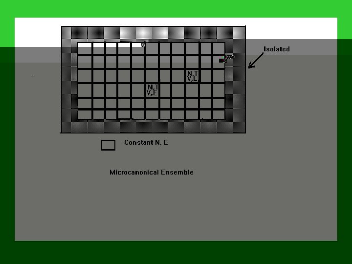
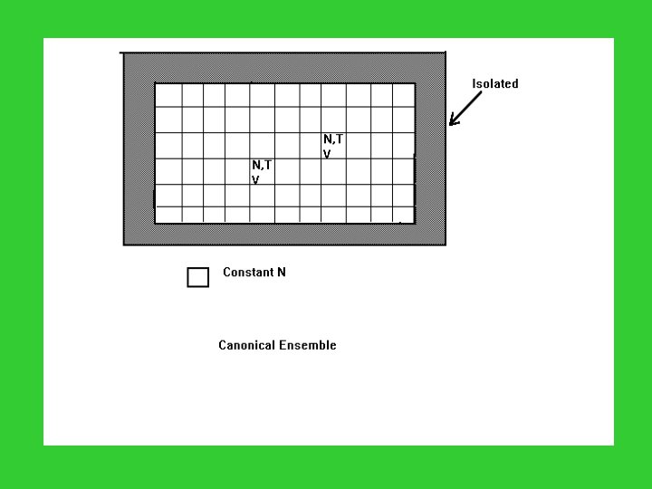
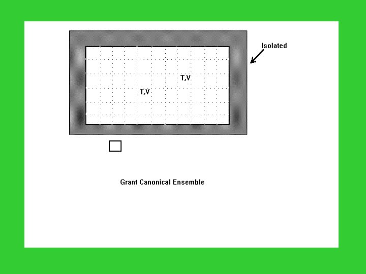
Microcanonical Ensemble: N, V, E are common; Canonical Ensemble: N, V, T are common; Grand Canonical Ensemble: , V, T are common. Microcanonical System: N, E are fixed; Canonical System: N is fixed, but E varies; Grand Canonical System: N, E vary.

Example: What kind of system is each of the following systems: (1) an isolated molecular system; (2) an equilibrium system enclosed by a heat conducting wall; (3) a pond; (4) a system surrounded by a rigid and insulating material.

Principle of Equal A Priori Probabilities of all accessible states of an isolated system are equal. For instance, four molecules in a three-level system: the following two conformations have the same probability. -----l-l---- 2 ---------l---------- 0 -----l----- 2 -----1 -1 -1 ---- ---------- 0

Configurations and Weights Imagine that an ensemble contains total A systems among which a 1 systems with energy E 1 and N 1 molecules, a 2 systems with energy E 2 and N 2 molecules, a 3 systems with energy E 3 and N 3 molecules, with energy 1, and so on. The specific distribution of systems in the ensemble is called configuration of the system, denoted as { a 1, a 2, a 3, . . . }.

A configuration { a 1, a 2, a 3, . . . } can be achieved in W different ways, where W is called the weight of the configuration. And W can be evaluated as follows, W = A! / (a 1! a 2! a 3!. . . ) Distribution of a Microcanonical Ensemble State Energy Occupation 1 E a 1 2 E a 2 3 E a 3 … … … k E ak … … …

Constraint i ai = A W = A! / a 1! a 2! a 3!… To maximize ln. W under the constraint, we construct a Lagrangian L = ln. W + i ai Thus, 0 = L/ ai = ln. W/ ai +

Utilizing the Stirling’s approximation, ln x! = x ln x - x ln. W/ ai = - ln ai/A = - , the probability of a system being found in state i, pi = ai/A = exp( ) = constant or, in another word, the probabilities of all states with the same energy are equal.

Distribution of a Canonical Ensemble State Energy Occupation 1 E 1 a 1 2 E 2 a 2 3 E 3 a 3 Constraints: i ai = A i ai Ei = … … … k Ek ak where, is the total energy in the ensemble. W = A! / a 1! a 2! a 3!… …

To maximize ln. W under the above constraints, construct a Lagrangian L = ln. W + i ai - i ai Ei 0 = L/ ai = ln. W/ ai + - Ei ln ai/A = - Ei the probability of a system being found in state i with the energy Ei , pi = ai/A = exp( - Ei)

The above formula is the canonical distribution of a system. Different from the Boltzmann distribution of independent molecules, the canonical distribution applies to an entire system as well as individual molecule. The molecules in this system can be independent of each other, or interact among themselves. Thus, the canonical distribution is more general than the Boltzmann distribution. (note, in the literature the canonical distribution and the Boltzmann distribution are sometimes interchangeable).

Distribution of a Grand Canonical Ensemble State Energy Mol. No. Occupation 1 E 1 N 1 a 1 2 E 2 N 2 a 2 3 E 3 N 3 a 3 … … k Ek Nk ak … …

Constraints: i ai = A i ai Ei = i ai Ni = N where, and N are the total energy and total number of molecules in the ensemble, respectively. W = A! / a 1!a 2! a 3!…

To maximize ln. W under the above constraints, construct a Lagrangian L = ln. W + i ai - i ai Ei - i ai Ni 0 = L/ ai = ln. W/ ai + - Ei - Ni ln ai/A = - Ei - Ni the probability of a system being found in state i with the energy Ei and the number of particles Ni, pi = ai/A = exp( - Ei - Ni)

The above formula describes the distribution of a grand canonical system, and is called the grand canonical distribution. When Ni is fixed, the above distribution becomes the canonical distribution. Thus, the grand canonical distribution is most general.

Quantum Statistics Quantum Particle: Fermion (S = 1/2, 3/2, 5/2, . . . ) e. g. electron, proton, neutron, 3 He nuclei Boson (S = 0, 1, 2, . . . ) e. g. deuteron, photon, phonon, 4 He nuclei Pauli Exclusion Principle: Two identical fermions can not occupy the same state at the same time. Question: what is the average number particles or occupation of a quantum state?

Fermi-Dirac Statistics System: a fermion’s state with an energy ( - / ) ---------l---- occupation n = 0 n = 1 energy 0 probability exp(0) exp[- ( - )]

There are only two states because of the Pauli exclusion principle. Thus, the average occupation of the quantum state , 1 / {exp[ ( - )] + 1}

Therefore, the average occupation number n( ) of a fermion state whose energy is , n( ) = 1 / {exp[ ( - )] + 1} is the chemical potential. When = , n = 1/2 For instance, distribution of electrons

Bose-Einstein Statistics System: a boson’s state with an energy Occupation of the system may be 0, 1, 2, 3, …, and correspondingly, the energy may be 0, , 2 , 3 , …. Therefore, the average occupation of the boson’s state,

= 1 / {exp[ ( - )] - 1} Therefore, the average occupation number n( ) of a boson state whose energy is , n( ) = 1 / {exp[ ( - )] - 1}

the chemical potential must less than or equal to the ground state energy of a boson, i. e. 0, where 0 is the ground state energy of a boson. This is because that otherwise there is a negative occupation which is not physical. When = 0, n( ) , i. e. , the occupation number is a macroscopic number. This phenomena is called Bose-Einstein Condensation! 4 He superfluid: when T T flows with no viscosity. 4 He fluid = 2. 17 K, c

Classical or Chemical Statistics When the temperature T is high enough or the density is very dilute, n( ) becomes very small, i. e. n( ) << 1. In another word, exp[ ( - )] >> 1. Neglecting +1 or -1 in the denominators, both Fermi-Dirac and Bose-Einstein Statistics become n( ) = exp[- ( - )] The Boltzmann distribution!

Canonical Partition Function the canonical distribution pi = exp(- - Ei) Sum over all the states, i pi = 1. Thus, pi = exp(- Ei) / Q where, Q i exp(- Ei) is called the canonical partition function.

An interpretation of the partition function: If we set the ground state energy E 0 to zero, As T 0, Q the number of ground state, usually 1; As T , Q the total number of states, usually .

Independent Molecules Total energy of a state i of the system, Ei = i(1) + i(2) + i(3) + i(4) +…+ i(N) Q = i exp[- i(1) - i(2) - i(3) - i(4) -… - i(N)] = { i exp[- i(1)]} { i exp[- i(2)]} … { i exp[- i(N)]} = q. N

Distinguishable and Indistinguishable Molecules for distinguishable molecules: Q = q. N N/N! Q = q for indistinguishable molecules:

Fundamental Thermodynamic Relationships Relation between energy and partition function U = U(0) - ( ln. Q/ )V The Relation between entropy S and partition function Q S = [U-U(0)] / T + k ln. Q The Helmholtz energy A - A(0) = -k. T ln Q

The Pressure p = -( A/ V)T p = k. T( ln. Q/ V)T The Enthalpy H - H(0) = -( ln. Q/ )V + k. TV( ln. Q/ V)T The Gibbs energy G - G(0) = - k. T ln Q + k. TV( ln. Q/ V)T

Non-Ideal Gas Now let’s derive the equation of state for real gases. Consider a real gas with N monatomic molecules in a volume V. Assuming the temperature is T, and the mass of each molecule is m. So the canonical partition function Q can be expressed as Q = i exp(-Ei / k. T) where the sum is over all possible state i, and Ei is the energy of state i.

In the classical limit, Q may be expressed as Q =(1/N!h 3 N) … exp(-H / k. T) dp 1 … dp. N dr 1 … dr. N where, H = (1/2 m) i pi 2 + i>j V(ri, rj) Q = (1/N!) (2 mk. T / h 2)3 N/2 ZN ZN = … exp(- i>j V(ri, rj) / k. T) dr 1 … dr. N ZN = VN , and [ note: for ideal gas, Z Q = (1/N!) (2 m k. T / h 2)3 N/2 VN ]

The equation of state may be obtained via p = k. T( ln. Q/ V)T We have thus, p / k. T = ( ln. Q/ V)T = (( ln. ZN N // V) V)TT ZN = … { 1 + [ exp(- i>j V(ri, rj) / k. T) - 1 ] } dr 1 … dr. N = VN + … [ exp(- i>j V(ri, rj) / k. T) - 1 ] dr 1 … dr. N VN + (1/2) VN-2 N(N-1) [ exp(- V(r 1, r 2) / k. T) - 1 ] dr 1 dr 2 VN { 1 - (1/2 V 2) N 2 [ 1 - exp(- V(r 1, r 2) / k. T) ] dr 1 dr 2 } = VN { 1 - B N 2 / V } where, B = (1/2 V) [ 1 - exp(- V(r 11, r 22) / k. T) ] dr 11 dr dr 22

Therefore, the equation of state for our gas: p / k. T = N / V + (N / V)2 B = n + B n 2 Comparison to the Virial Equation of State The equation of state for a real gas P / k. T = n + B 2(T) n 2 + B 3(T) n 3 + … This is the virial equation of state, and the quantities B 2(T), B 3(T), … are called the second, third, … virial coefficients.

Thus,

A. HARD-SPHERE POTENTIAL U(r 12) = r 12 < 0 r 12 > = (1/2) 00 4 r 22 dr dr B 2(T) = (1/2) 3/3 = 2 3/3

B. SQUARE-WELL POTENTIAL U(r 12) = - 0 r 12 < < r 12 < r 12 > = (1/2) 00 4 r B 2(T) = (1/2) 4 r 22 dr dr = (2 33/3) [1 - ( 33 -1) ( e - 1 )]

C. LENNARD-JONES POTENTIAL U(r) = 4 [ ( /r)12 - ( /r)6 ] B 2(T) = ( ) 0 { 1 - exp{( ) [ ]} } 4 r 2 dr With x = /r, T* = k. T / = 0 { 1 - exp[(-4/T*) ( x 12 - x 6 )] } x 2 dx

Maxwell’s Demon (1867)

Thermal Fluctuation (Smolochowski, 1912) In his talk “Experimentally Verifiable Molecular Phenomena that Contradict Ordinary Thermodynamics”, … Smoluchowski showed That one could observe violations of almost all the usual statements Of the second law by dealing with sufficiently small systems. … the increase of entropy… The one statement that could be upheld… was the impossibility of perpetual motion of the second kind. No device could be ever made that would use the existing fluctuations to convert heat completely into work on a macroscopic scale … subject to the same chance fluctuations…. -----H. S. Leff & A. F. Rex, “Maxwell’s Demon”

Szilard’s one-molecule gas model (1929) To save the second law, a measure of where-about of the molecule produces at least entropy > k ln 2

Measurement via light signals (L. Brillouin, 1951) h >> k T A Temporary Resolution !!!? ? ?

Mechanical Detection of the Molecule Counter-clockwise rotation always !!! A Perpetual Machine of second kind ? ? ?

Bennett’s solution (1982) To complete thermodynamic circle, Demon has to erase its memory !!! Memory eraser needs minimal Entropy production of k ln 2 (R. Landauer, 1961) Demon’s memory

Feynman’s Ratchet and Pawl System (1961) T 1=T 2, no net rotation Feynman’s Lecture Notes

A honeybee stinger potential coordinate

A Simplest Maxwell’s demon door

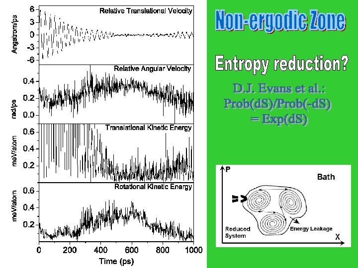
Average over 200 trajectories No temperature difference!!! T t

A cooler demon T 1 > T 2 door TL > TR !!!

TL TR Number of particles in left side Our simple demon No. of particles: 60 The door’s moment of inertia: 0. 2 Force constant of the string: 10 Maxwell’s demon No. of particles: 60 Threshold energy: 20

Feynman’s Ratchet and Pawl System (1961) T 1=T 2, no net rotation T 1 > T 2, counter-clockwise rotation T 1 > T 2, clockwise rotation Feynman’s Lecture Notes rate Mechanical Rectifier

A two-chamber design: an analogy to Feynman’s Ratchet and Pawl string Feynman’s Lecture Notes Our two-chamber design

Potential of the pawl string potential radian

Feynman’s ratchet-pawl system

Feynman’s Ratchet and Pawl TL = T B

Micro-reversibility Pawl a transition state

Determination of temperature at equilibrium

Simulation results The ratchet moves when the leg is cooled down.

radian Angular velocity versus TL - TB k. B

The Ratchet and Pawl as an engine TB=80 TL=20 (TB- TL) / TL =75%

Density of distribution in the phase space N = r(q 1…qf, p 1…pf) q 1. . . qf p 1. . . pf where r(q 1…qf, p 1…pf) is fine-grained density at (q 1…qf, p 1…pf) Liouville’s Theorem: dr/dt = 0 Coarse-grained density over q 1. . . qf p 1. . . pf at (q 1…qf, p 1…pf) : P = … r(q 1…qf, p 1…pf) dq 1. . . dqf dp 1. . . dpf / q 1. . . qf p 1. . . pf Boltzmann’s H: H = … P log P dq 1. . . dqf dp 1. . . dpf

Boltzmann’s H-Theorem d( … r log r dq 1. . . dqf dp 1. . . dpf)/dt = 0 Q = r log r - r log P - r + P 0 At t 1, r 1 = P 1 H 1= … r 1 log r 1 dq 1. . . dqf dp 1. . . dpf At t 2, r 2 P 2 H 2= … P 2 log P 2 dq 1. . . dqf dp 1. . . dpf H 1 - H 2 0

Oscillation Hibernation Revival

Revival Hibernation Entropy [Q: Partition Function] S = k ln. W = - Nk i pi ln pi = k ln. Q - ( ln. Q/ )V / T