Thu AM Part 5 Advanced control case studies

Thu AM Part 5: Advanced control + case studies Advanced control layer (1 h) • Design based on simple elements: – – – – • Ratio control Cascade control Selectors Input resetting (valve position control) Split range control Decouplers (including phsically based) When should these elements be used? When use MPC instead? Case studies (3 h) • Example: Distillation column control • Example: Plantwide control of complete plant Recycle processes: How to avoid snowballing 1

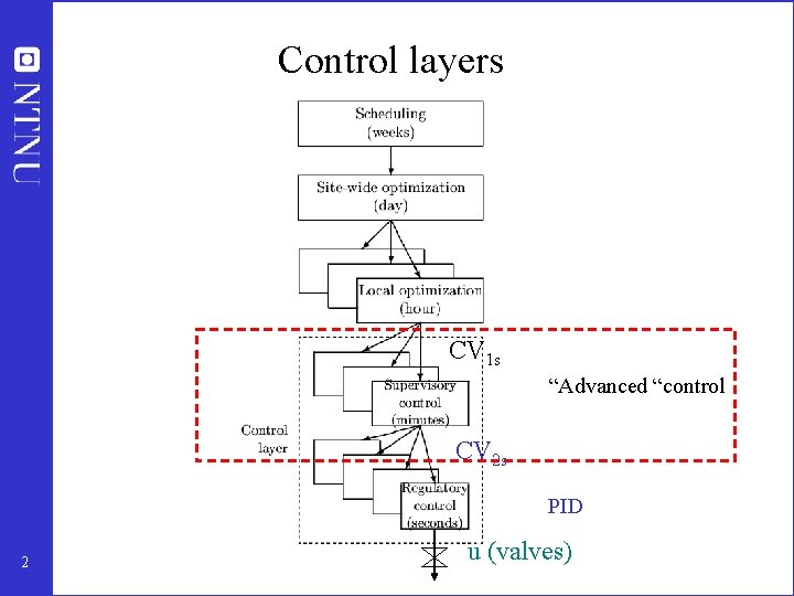
Control layers CV 1 s “Advanced “control CV 2 s PID 2 u (valves)

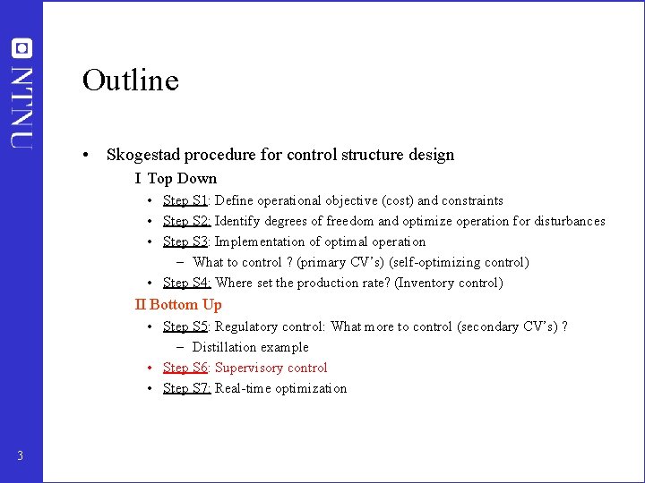
Outline • Skogestad procedure for control structure design I Top Down • Step S 1: Define operational objective (cost) and constraints • Step S 2: Identify degrees of freedom and optimize operation for disturbances • Step S 3: Implementation of optimal operation – What to control ? (primary CV’s) (self-optimizing control) • Step S 4: Where set the production rate? (Inventory control) II Bottom Up • Step S 5: Regulatory control: What more to control (secondary CV’s) ? – Distillation example • Step S 6: Supervisory control • Step S 7: Real-time optimization 3

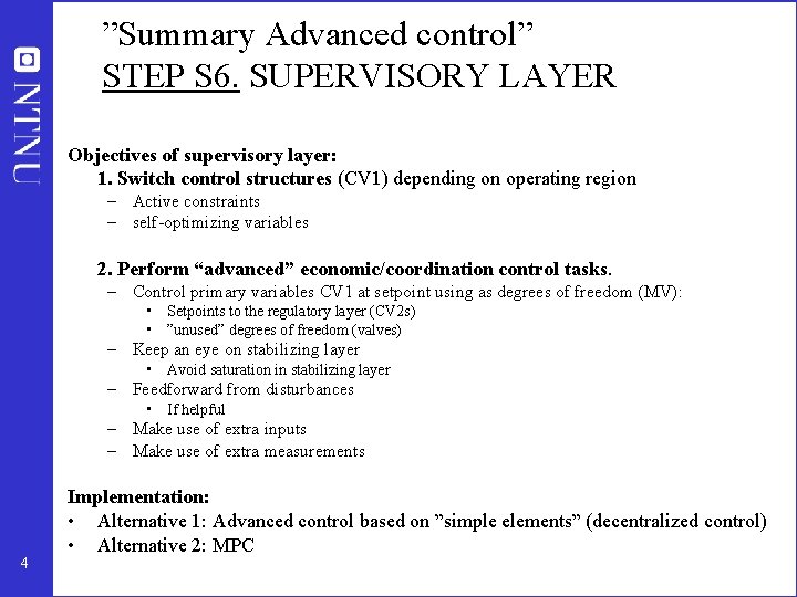
”Summary Advanced control” STEP S 6. SUPERVISORY LAYER Objectives of supervisory layer: 1. Switch control structures (CV 1) depending on operating region – Active constraints – self-optimizing variables 2. Perform “advanced” economic/coordination control tasks. – Control primary variables CV 1 at setpoint using as degrees of freedom (MV): • Setpoints to the regulatory layer (CV 2 s) • ”unused” degrees of freedom (valves) – Keep an eye on stabilizing layer • Avoid saturation in stabilizing layer – Feedforward from disturbances • If helpful – Make use of extra inputs – Make use of extra measurements 4 Implementation: • Alternative 1: Advanced control based on ”simple elements” (decentralized control) • Alternative 2: MPC

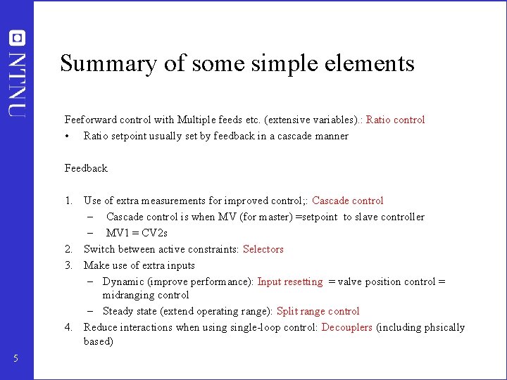
Summary of some simple elements Feeforward control with Multiple feeds etc. (extensive variables). : Ratio control • Ratio setpoint usually set by feedback in a cascade manner Feedback 1. Use of extra measurements for improved control; : Cascade control – Cascade control is when MV (for master) =setpoint to slave controller – MV 1 = CV 2 s 2. Switch between active constraints: Selectors 3. Make use of extra inputs – Dynamic (improve performance): Input resetting = valve position control = midranging control – Steady state (extend operating range): Split range control 4. Reduce interactions when usingle-loop control: Decouplers (including phsically based) 5

Control configuration elements • Control configuration. The restrictions imposed on the overall controller by decomposing it into a set of local controllers (subcontrollers, units, elements, blocks) with predetermined links and with a possibly predetermined design sequence where subcontrollers are designed locally. Some control configuration elements: • Cascade controllers • Decentralized controllers • Feedforward elements • Decoupling elements • Input resetting/Valve position control/Midranging control • Split-range control • Selectors 6

Most important control structures 1. 2. 3. 7 Feedback control Ratio control (special case of feedforward) Cascade control

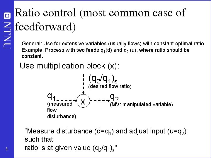
Ratio control (most common case of feedforward) General: Use for extensive variables (usually flows) with constant optimal ratio Example: Process with two feeds q 1(d) and q 2 (u), where ratio should be constant. Use multiplication block (x): (q 2/q 1)s (desired flow ratio) q 1 (measured flow disturbance) 8 x q 2 (MV: manipulated variable) “Measure disturbance (d=q 1) and adjust input (u=q 2) such that ratio is at given value (q 2/q 1)s”

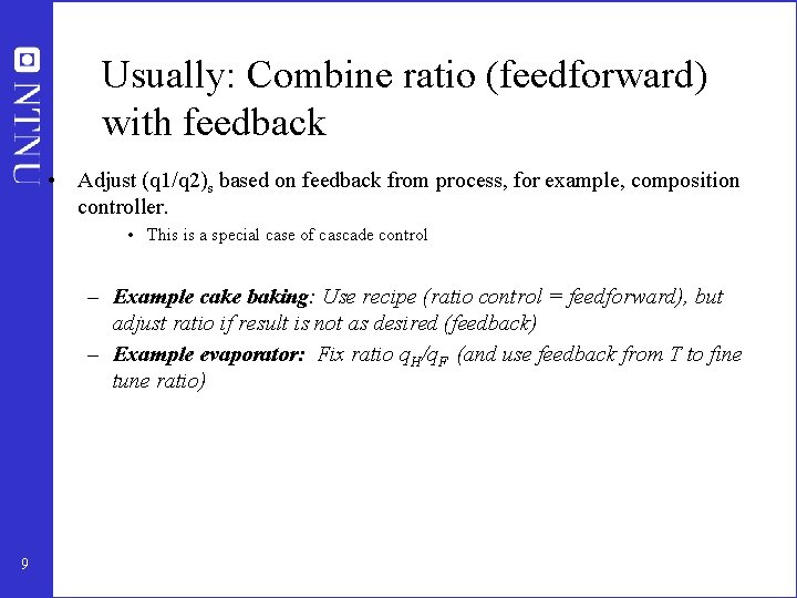
Usually: Combine ratio (feedforward) with feedback • Adjust (q 1/q 2)s based on feedback from process, for example, composition controller. • This is a special case of cascade control – Example cake baking: Use recipe (ratio control = feedforward), but adjust ratio if result is not as desired (feedback) – Example evaporator: Fix ratio q. H/q. F (and use feedback from T to fine tune ratio) 9

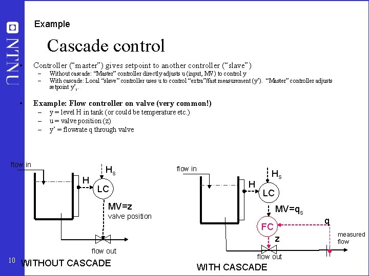
Example Cascade control • Controller (“master”) gives setpoint to another controller (“slave”) – – • Without cascade: “Master” controller directly adjusts u (input, MV) to control y With cascade: Local “slave” controller uses u to control “extra”/fast measurement (y’). “Master” controller adjusts setpoint y’s. Example: Flow controller on valve (very common!) – – – y = level H in tank (or could be temperature etc. ) u = valve position (z) y’ = flowrate q through valve flow in H Hs LC MV=z MV=qs valve position FC z flow out 10 WITHOUT CASCADE flow out WITH CASCADE q measured flow

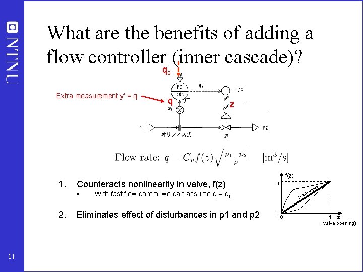
What are the benefits of adding a flow controllerq (inner cascade)? s Extra measurement y’ = q 1. 11 z Counteracts nonlinearity in valve, f(z) • 2. q f(z) 1 v ar With fast flow control we can assume q = qs Eliminates effect of disturbances in p 1 and p 2 e alv e lin 0 0 1 z (valve opening)

Example (again): Evaporator with heating From reactor q. F [m 3/s] TF [K] c. F [mol/m 3] evaporation level measurement temperature measurement T ∞ H q [m 3/s] T [K] c [mol/m 3] Heating fluid q. H [m 3/s] TH [K] concentrate NEW Control objective • Keep level H at desired value • Keep composition c (rather than temperature T) at desired value BUT: Composition measurement has large delay + unreliable Suggest control structure based on cascade control 12

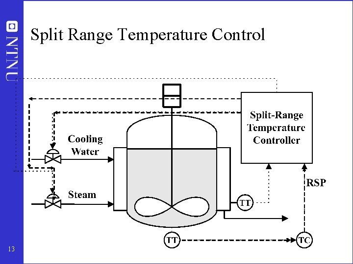
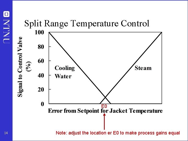
Split Range Temperature Control 13

Split Range Temperature Control E 0 14 Note: adjust the location er E 0 to make process gains equal

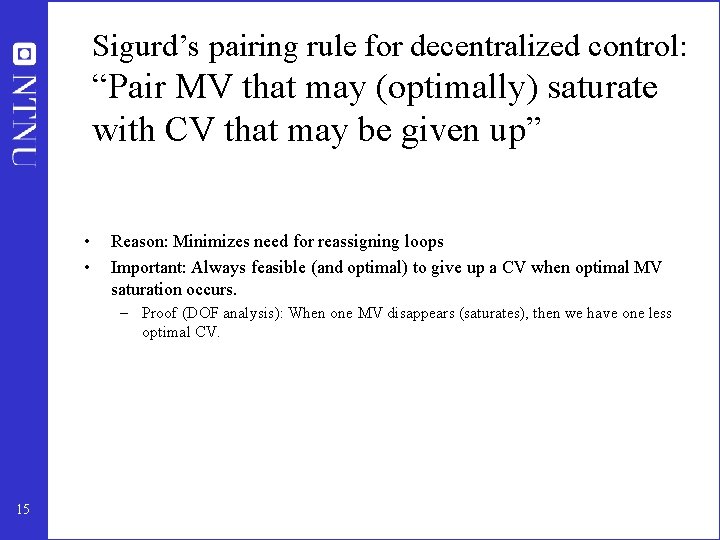
Sigurd’s pairing rule for decentralized control: “Pair MV that may (optimally) saturate with CV that may be given up” • • Reason: Minimizes need for reassigning loops Important: Always feasible (and optimal) to give up a CV when optimal MV saturation occurs. – Proof (DOF analysis): When one MV disappears (saturates), then we have one less optimal CV. 15

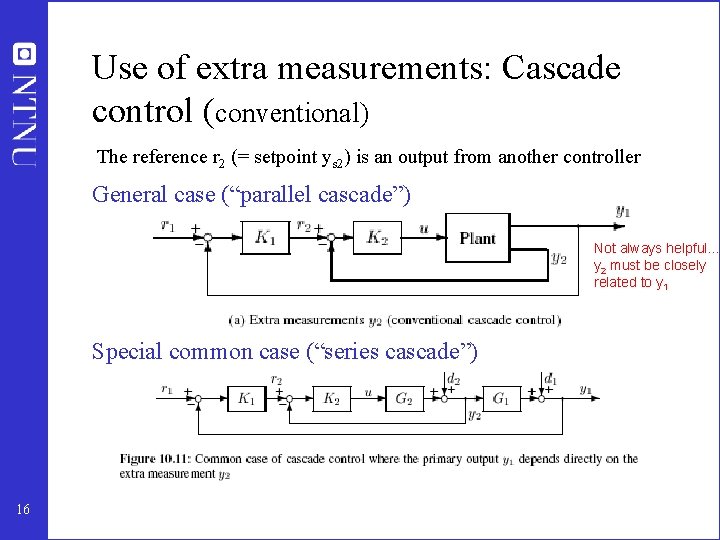
Use of extra measurements: Cascade control (conventional) The reference r 2 (= setpoint ys 2) is an output from another controller General case (“parallel cascade”) Not always helpful… y 2 must be closely related to y 1 Special common case (“series cascade”) 16

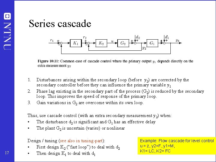
Series cascade 1. 2. 3. Disturbances arising within the secondary loop (before y 2) are corrected by the secondary controller before they can influence the primary variable y 1 Phase lag existing in the secondary part of the process (G 2) is reduced by the secondary loop. This improves the speed of response of the primary loop. Gain variations in G 2 are overcome within its own loop. Thus, use cascade control (with an extra secondary measurement y 2) when: • The disturbance d 2 is significant and G 1 has an effective delay • The plant G 2 is uncertain (varies) or nonlinear 17 Design / tuning (see also in tuning-part): • First design K 2 (“fast loop”) to deal with d 2 • Then design K 1 to deal with d 1 Example: Flow cascade for level control u = z, y 2=F, y 1=M, K 1= LC, K 2= FC

Pressure control distillation • Need to stabilze p using Qc • But want Qc to be max • Use cascade with backoff on Qc ( • Another similar example: reactor temperature control (stabilization) closed to Qmax. 18

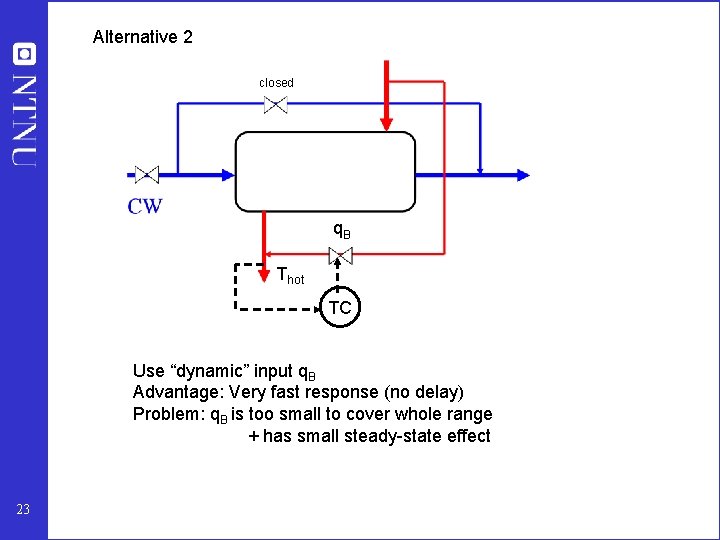
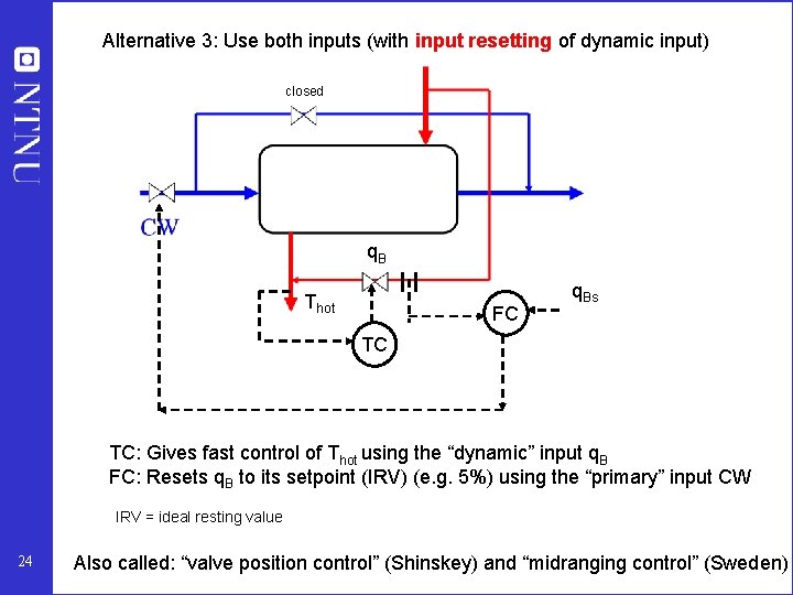
Use of extra inputs Two different cases 1. Have extra dynamic inputs (degrees of freedom) Cascade implementation: “Input resetting to ideal resting value” Example: Heat exchanger with extra bypass Also known as: Midranging control, valve position control 2. Need several inputs to cover whole range (because primary input may saturate) (steady-state) Split-range control Example 1: Control of room temperature using AC (summer), heater (winter), fireplace (winter cold) Example 2: Pressure control using purge and inert feed (distillation) 19

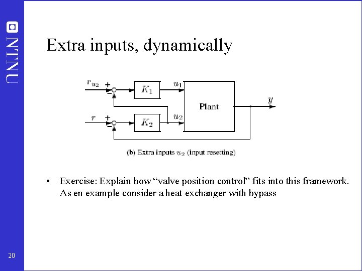
Extra inputs, dynamically • Exercise: Explain how “valve position control” fits into this framework. As en example consider a heat exchanger with bypass 20

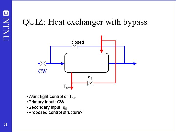
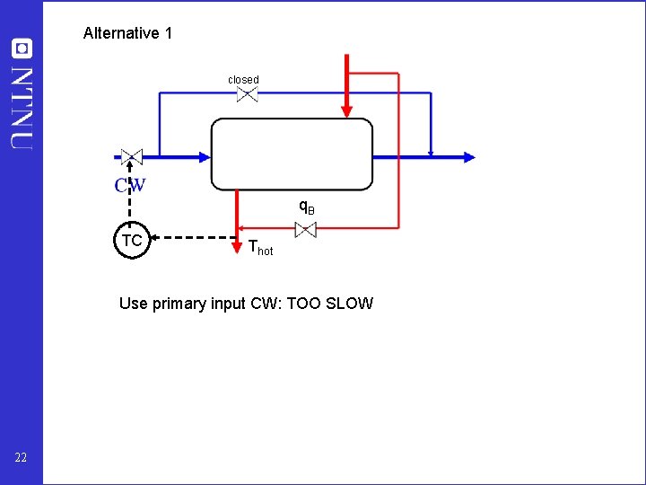
QUIZ: Heat exchanger with bypass closed q. B Thot • Want tight control of Thot • Primary input: CW • Secondary input: q. B • Proposed control structure? 21

Alternative 1 closed q. B TC Thot Use primary input CW: TOO SLOW 22

Alternative 2 closed q. B Thot TC Use “dynamic” input q. B Advantage: Very fast response (no delay) Problem: q. B is too small to cover whole range + has small steady-state effect 23

Alternative 3: Use both inputs (with input resetting of dynamic input) closed q. B Thot FC q. Bs TC TC: Gives fast control of Thot using the “dynamic” input q. B FC: Resets q. B to its setpoint (IRV) (e. g. 5%) using the “primary” input CW IRV = ideal resting value 24 Also called: “valve position control” (Shinskey) and “midranging control” (Sweden)

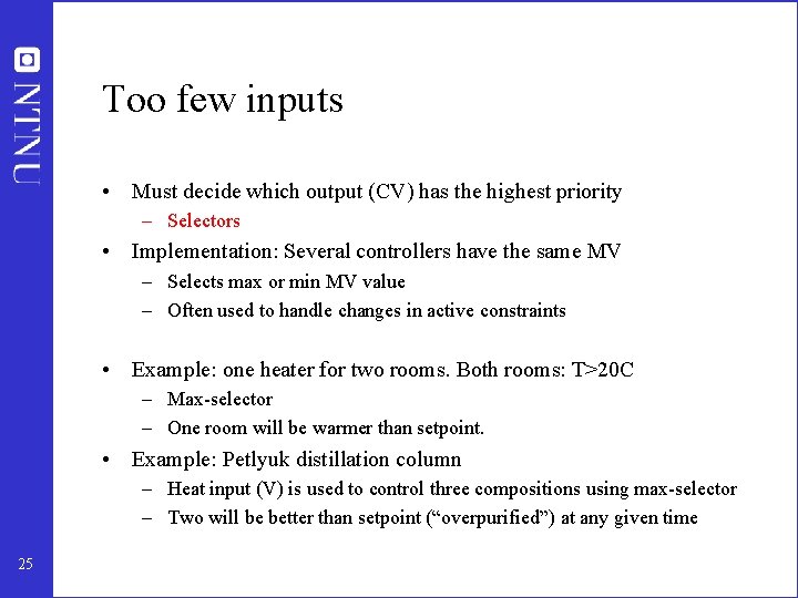
Too few inputs • Must decide which output (CV) has the highest priority – Selectors • Implementation: Several controllers have the same MV – Selects max or min MV value – Often used to handle changes in active constraints • Example: one heater for two rooms. Both rooms: T>20 C – Max-selector – One room will be warmer than setpoint. • Example: Petlyuk distillation column – Heat input (V) is used to control three compositions using max-selector – Two will be better than setpoint (“overpurified”) at any given time 25

Divided wall column example 26

Control of primary variables • Purpose: Keep primary controlled outputs c=y 1 at optimal setpoints cs • Degrees of freedom: Setpoints y 2 s in reg. control layer • Main structural issue: Decentralized or multivariable? 27

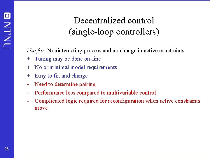
Decentralized control (single-loop controllers) Use for: Noninteracting process and no change in active constraints + Tuning may be done on-line + No or minimal model requirements + Easy to fix and change - Need to determine pairing - Performance loss compared to multivariable control - Complicated logic required for reconfiguration when active constraints move 28

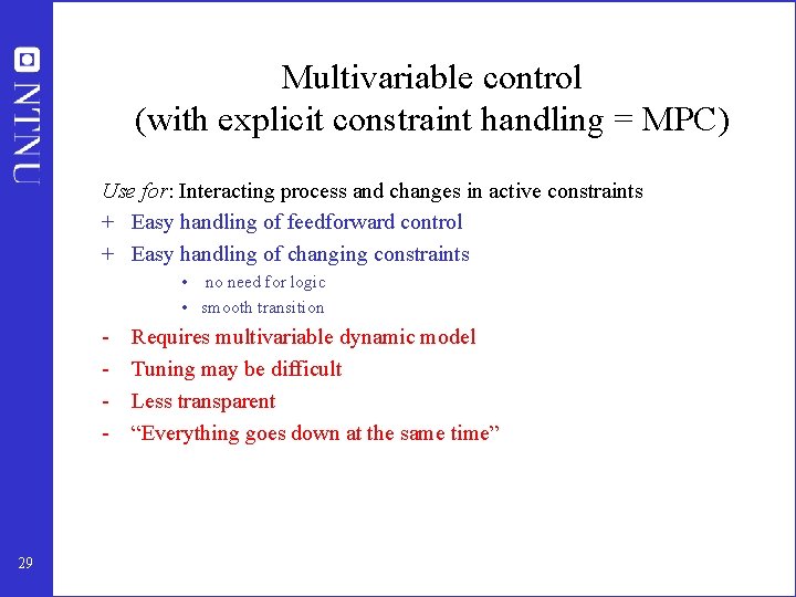
Multivariable control (with explicit constraint handling = MPC) Use for: Interacting process and changes in active constraints + Easy handling of feedforward control + Easy handling of changing constraints • no need for logic • smooth transition - 29 Requires multivariable dynamic model Tuning may be difficult Less transparent “Everything goes down at the same time”

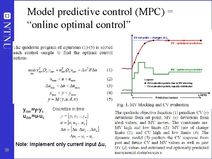
Model predictive control (MPC) = “online optimal control” ydev=y-ys udev=u-us 30 Discretize in time: Note: Implement only current input Δu 1

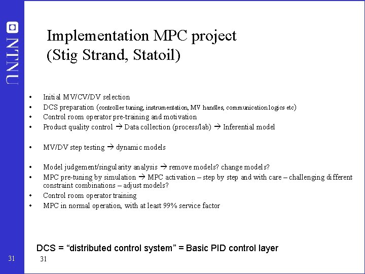
Implementation MPC project (Stig Strand, Statoil) • • Initial MV/CV/DV selection DCS preparation (controller tuning, instrumentation, MV handles, communication logics etc) Control room operator pre-training and motivation Product quality control Data collection (process/lab) Inferential model • MV/DV step testing dynamic models • • Model judgement/singularity analysis remove models? change models? MPC pre-tuning by simulation MPC activation – step by step and with care – challenging different constraint combinations – adjust models? Control room operator training MPC in normal operation, with at least 99% service factor • • DCS = “distributed control system” = Basic PID control layer 31 31

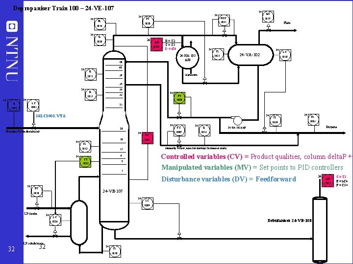
Depropaniser Train 100 – 24 -VE-107 24 24 24 PI PC 1020 1014 24 24 TI 24 1020 AR 1008 B = C 2 C = C 3 D = i. C 4 24 24 -HA-103 A/B 48 PDC 1021 TI 1021 HC 1015 Flare 24 24 -VA-102 LC 1010 40 24 TI Kjølevann 39 1011 35 24 34 TI 24 33 1017 24 24 LC 1001 TI 1005 FC 1008 21 24 LC 1001. VYA 24 24 20 Bottoms from deetaniser 24 24 18 FC 1009 24 TI 25 FI 1003 Propane 24 -PA-102 A/B 1013 1009 TI 1012 24 PD TI 1038 Normally 0 flow, used for start-ups to remove inerts 17 Controlled variables (CV) = Product qualities, column delta. P ++ Manipulated variables (MV) = Set points to PID controllers 6 TC 1022 5 1 Disturbance variables (DV) = Feedforward 24 PC 24 -VE-107 1010 24 LC 1009 LP steam 24 LC Debutaniser 24 -VE-108 1026 LP condensate 32 32 24 TI 1018 24 AR 1005 C = C 3 E = n. C 4 F = C 5+

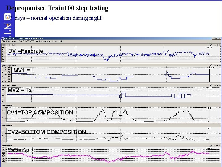
Depropaniser Train 100 step testing • 3 days – normal operation during night • DV =Feedrate MV 1 = L MV 2 = Ts CV 1=TOP COMPOSITION CV 2=BOTTOM COMPOSITION CV 3=¢p 33 33

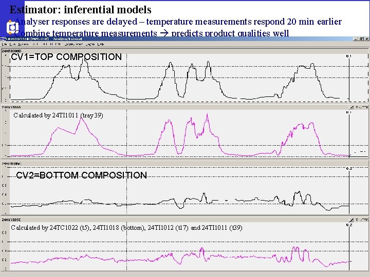
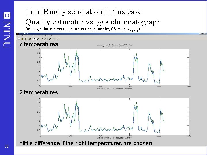
Estimator: inferential models • Analyser responses are delayed – temperature measurements respond 20 min earlier • Combine temperature measurements predicts product qualities well CV 1=TOP COMPOSITION Calculated by 24 TI 1011 (tray 39) CV 2=BOTTOM COMPOSITION Calculated by 24 TC 1022 (t 5), 24 TI 1018 (bottom), 24 TI 1012 (t 17) and 24 TI 1011 (t 39) 34 34

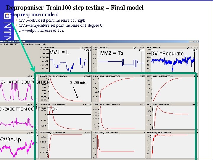
Depropaniser Train 100 step testing – Final model • Step response models: • MV 1=reflux set point increase of 1 kg/h • MV 2=temperature set point increase of 1 degree C • DV=output increase of 1%. MV 1 = L CV 1=TOP COMPOSITION CV 2=BOTTOM COMPOSITION CV 3=¢p 35 35 MV 2 = Ts 3 t 20 min DV =Feedrate

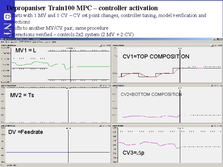
Depropaniser Train 100 MPC – controller activation • Starts with 1 MV and 1 CV – CV set point changes, controller tuning, model verification and corrections • Shifts to another MV/CV pair, same procedure • Interactions verified – controls 2 x 2 system (2 MV + 2 CV) • Expects 3 – 5 days tuning with set point changes to achieve satisfactory performance MV 1 = L CV 1=TOP COMPOSITION MV 2 = Ts CV 2=BOTTOM COMPOSITION DV =Feedrate 36 36 CV 3=¢p

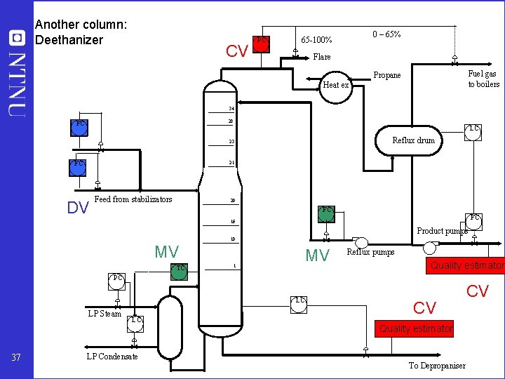
Another column: Deethanizer CV PC 0 – 65% 65 -100% Flare Fuel gas to boilers Propane Heat ex 34 28 FC LC Reflux drum 23 FC 21 DV Feed from stabilizators 20 FC FC 16 Product pumps 10 MV TC MV 1 Reflux pumps Quality estimator PC LC LP Steam 37 LC LP Condensate CV Quality estimator To Depropaniser CV

Top: Binary separation in this case Quality estimator vs. gas chromatograph (use logarithmic composition to reduce nonlinearity, CV = - ln ximpurity) 7 temperatures 2 temperatures 38 =little difference if the right temperatures are chosen

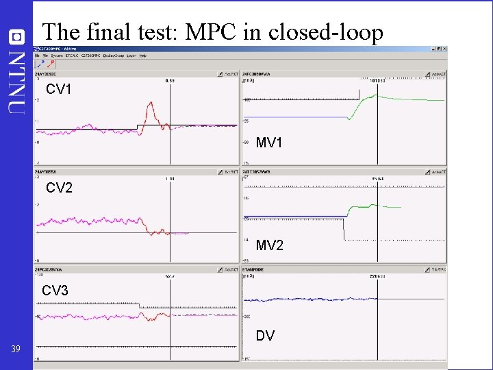
The final test: MPC in closed-loop CV 1 MV 1 CV 2 MV 2 CV 3 DV 39

Conclusion MPC • Generally simpler than previous advanced control • Well accepted by operators • Statoil: Use of in-house technology and expertise successful 40

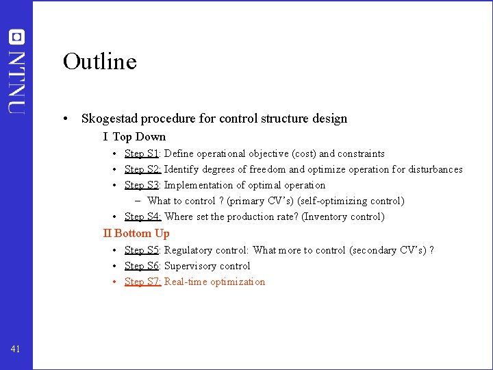
Outline • Skogestad procedure for control structure design I Top Down • Step S 1: Define operational objective (cost) and constraints • Step S 2: Identify degrees of freedom and optimize operation for disturbances • Step S 3: Implementation of optimal operation – What to control ? (primary CV’s) (self-optimizing control) • Step S 4: Where set the production rate? (Inventory control) II Bottom Up • Step S 5: Regulatory control: What more to control (secondary CV’s) ? • Step S 6: Supervisory control • Step S 7: Real-time optimization 41

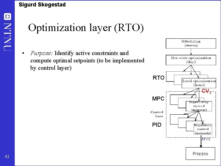
Sigurd Skogestad Optimization layer (RTO) • Purpose: Identify active constraints and compute optimal setpoints (to be implemented by control layer) RTO CVs MPC PID MVs 42 Process

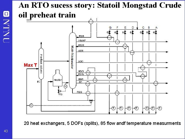
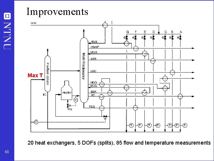
An RTO sucess story: Statoil Mongstad Crude oil preheat train Max T 20 heat exchangers, 5 DOFs (splits), 85 flow andf temperature measurments 43

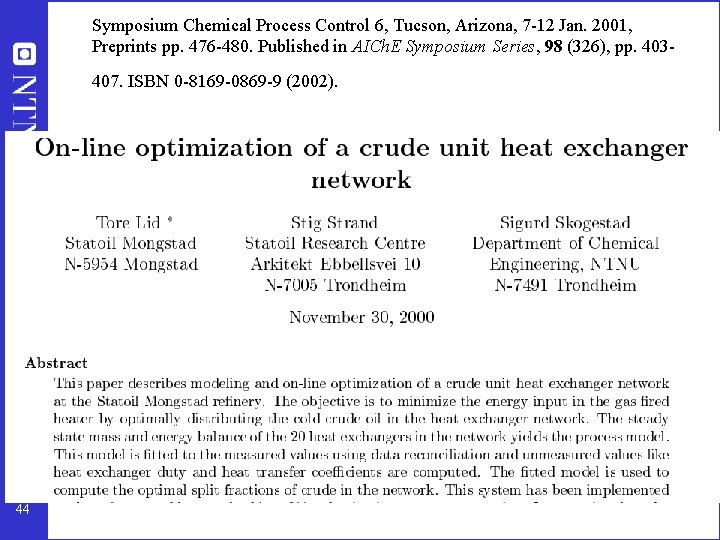
Symposium Chemical Process Control 6, Tucson, Arizona, 7 -12 Jan. 2001, Preprints pp. 476 -480. Published in AICh. E Symposium Series, 98 (326), pp. 403407. ISBN 0 -8169 -0869 -9 (2002). 44

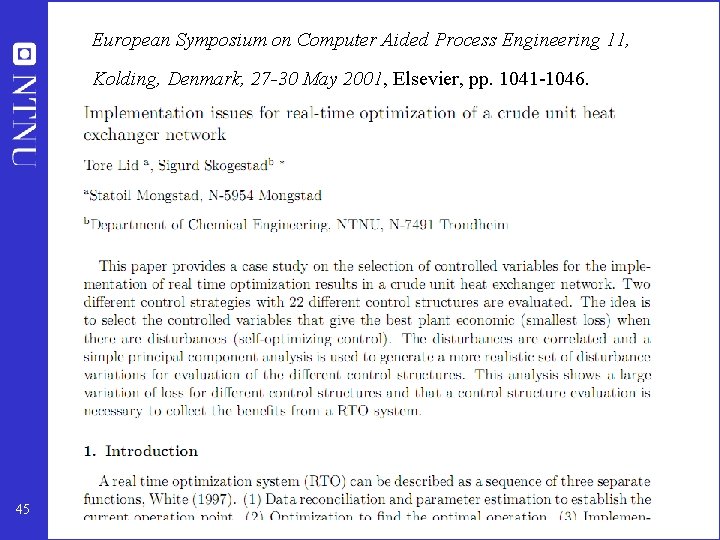
European Symposium on Computer Aided Process Engineering 11, Kolding, Denmark, 27 -30 May 2001, Elsevier, pp. 1041 -1046. 45

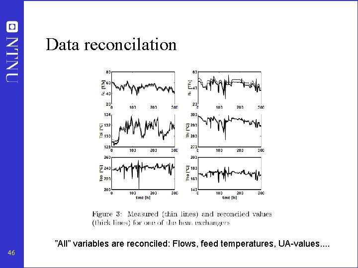
Data reconcilation ”All” variables are reconciled: Flows, feed temperatures, UA-values. . 46

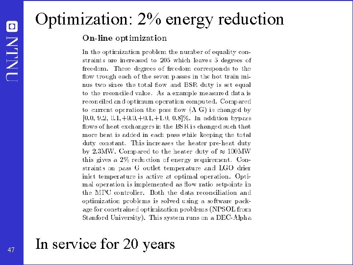
Optimization: 2% energy reduction 47 In service for 20 years

Improvements Max T 20 heat exchangers, 5 DOFs (splits), 85 flow and temperature measurements 48

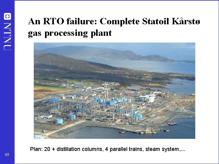
An RTO failure: Complete Statoil Kårstø gas processing plant Plan: 20 + distillation columns, 4 parallel trains, steam system, . . . 49

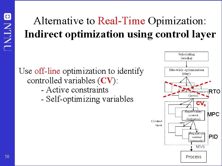
Alternative to Real-Time Opimization: Indirect optimization using control layer Use off-line optimization to identify controlled variables (CV): - Active constraints - Self-optimizing variables RTO CVs MPC PID MVs 50 Process

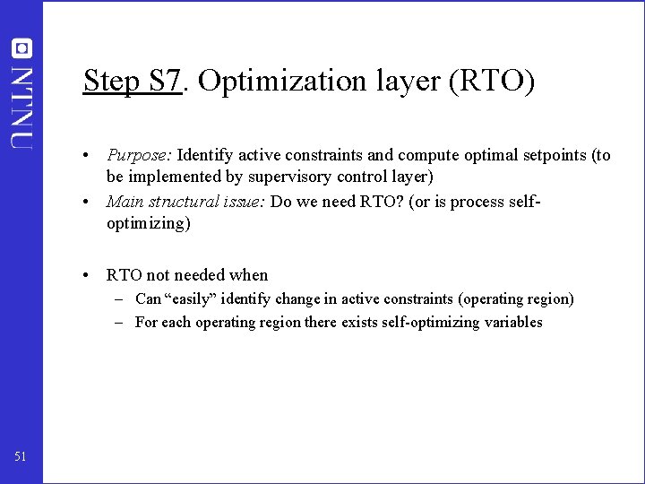
Step S 7. Optimization layer (RTO) • Purpose: Identify active constraints and compute optimal setpoints (to be implemented by supervisory control layer) • Main structural issue: Do we need RTO? (or is process selfoptimizing) • RTO not needed when – Can “easily” identify change in active constraints (operating region) – For each operating region there exists self-optimizing variables 51

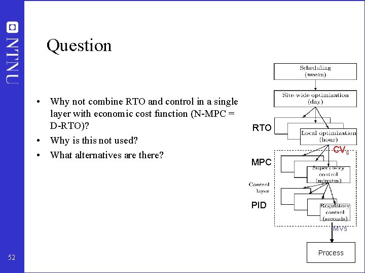
Question • Why not combine RTO and control in a single layer with economic cost function (N-MPC = D-RTO)? • Why is this not used? • What alternatives are there? RTO CVs MPC PID MVs 52 Process