Inverse Compositional Spatial Transformer Networks ChenHsuan Lin Simon

Inverse Compositional Spatial Transformer Networks Chen-Hsuan Lin, Simon Lucey Carnegie Mellon University

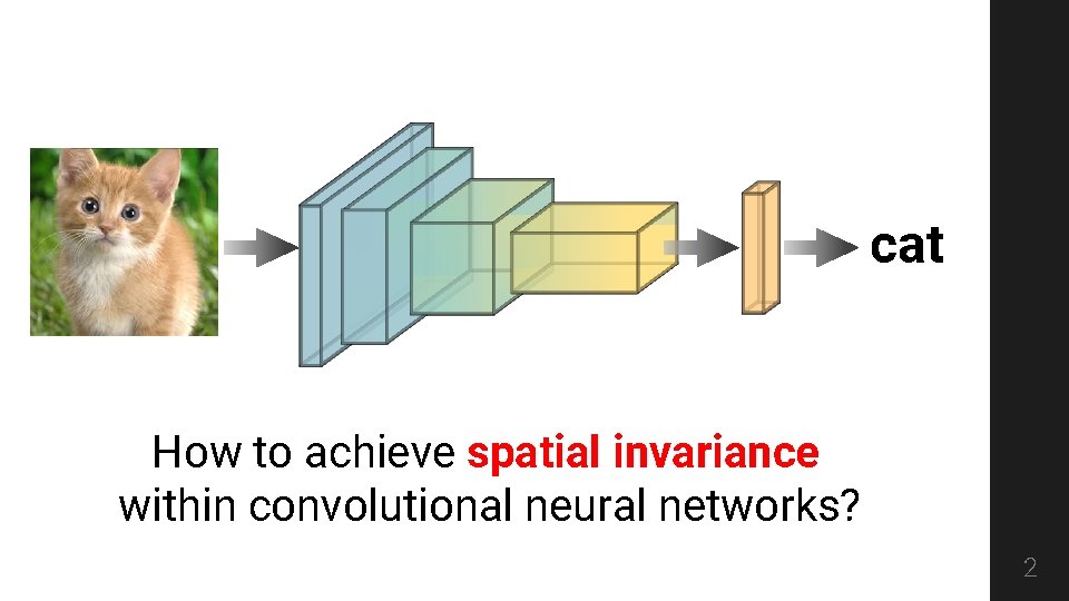
cat How to achieve spatial invariance within convolutional neural networks? 2

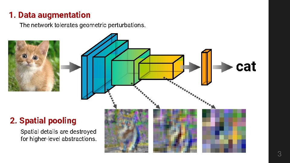
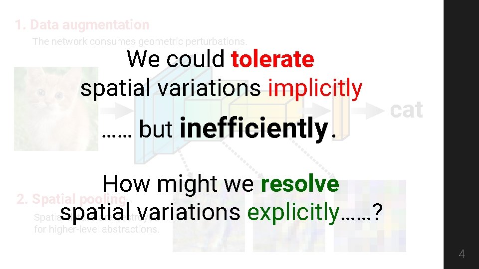
1. Data augmentation The network tolerates geometric perturbations. cat 2. Spatial pooling Spatial details are destroyed for higher-level abstractions. 3

1. Data augmentation The network consumes geometric perturbations. We could tolerate spatial variations implicitly …… but inefficiently. cat How might we resolve 2. Spatial pooling variations explicitly……? Spatialspatial details are destroyed for higher-level abstractions. 4

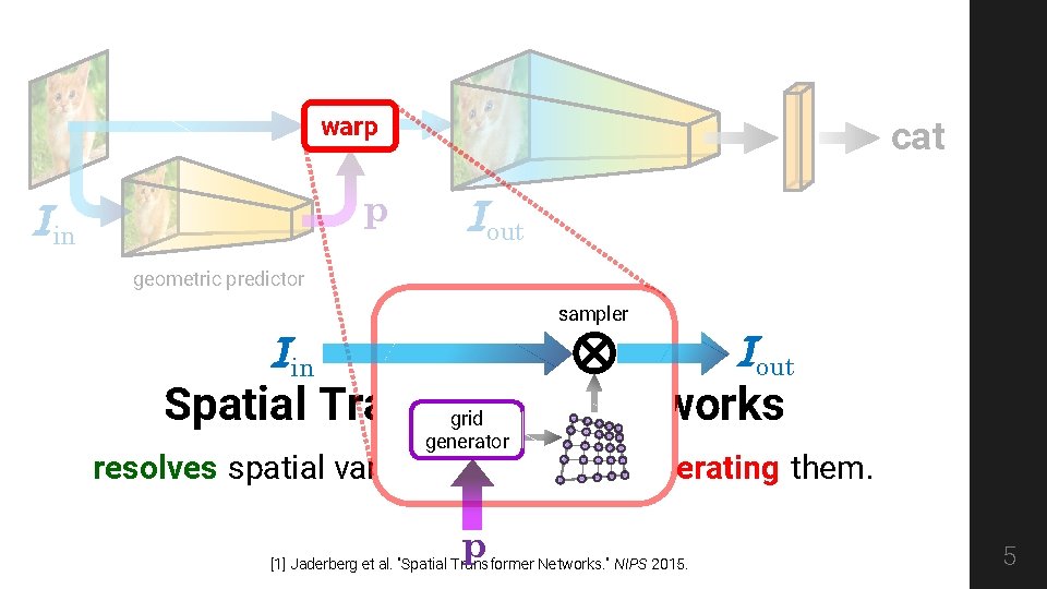
warp p Iin cat Iout geometric predictor sampler Iout Iin Spatial Transformer Networks grid generator resolves spatial variations instead of tolerating them. p [1] Jaderberg et al. "Spatial Transformer Networks. " NIPS 2015. 5

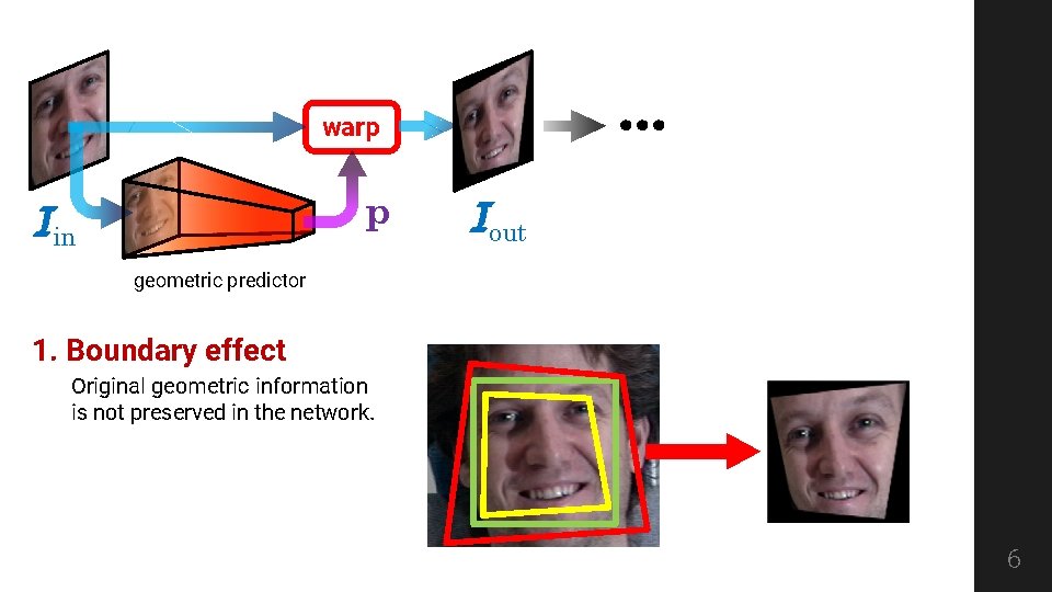
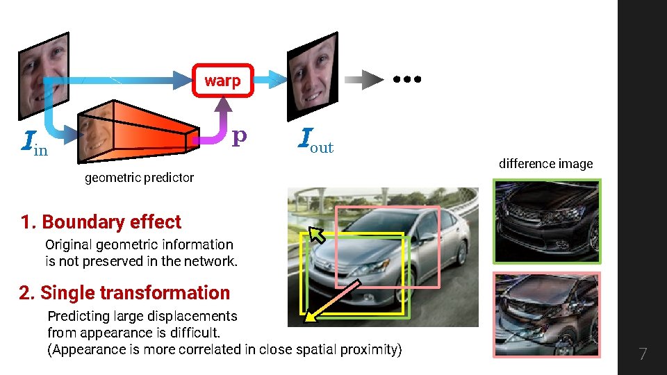
… warp p Iin Iout geometric predictor 1. Boundary effect Original geometric information is not preserved in the network. 6

… warp p Iin Iout geometric predictor difference image 1. Boundary effect Original geometric information is not preserved in the network. 2. Single transformation Predicting large displacements from appearance is difficult. (Appearance is more correlated in close spatial proximity) 7

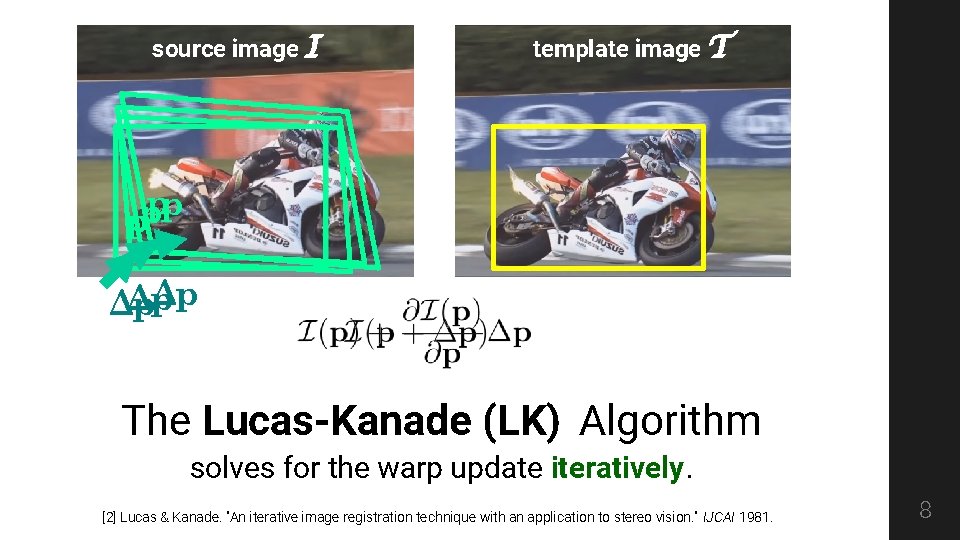
source image I template image T p p Δp Δp Δp The Lucas-Kanade (LK) Algorithm solves for the warp update iteratively. [2] Lucas & Kanade. "An iterative image registration technique with an application to stereo vision. " IJCAI 1981. 8

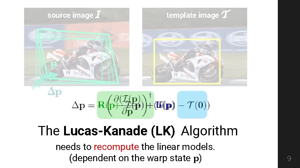
source image I template image T p Δp The Lucas-Kanade (LK) Algorithm needs to recompute the linear models. (dependent on the warp state p) 9

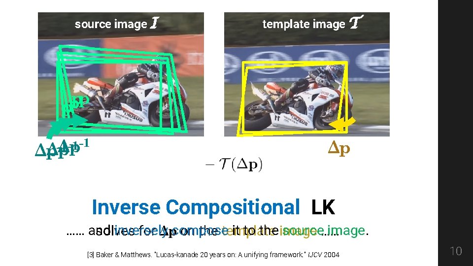
source image I template image T p p -1 -1 -1 Δp Δp Inverse Compositional LK …… and inversely it to the image source…… image. solves for Δpcompose on the template [3] Baker & Matthews. "Lucas-kanade 20 years on: A unifying framework. " IJCV 2004 10

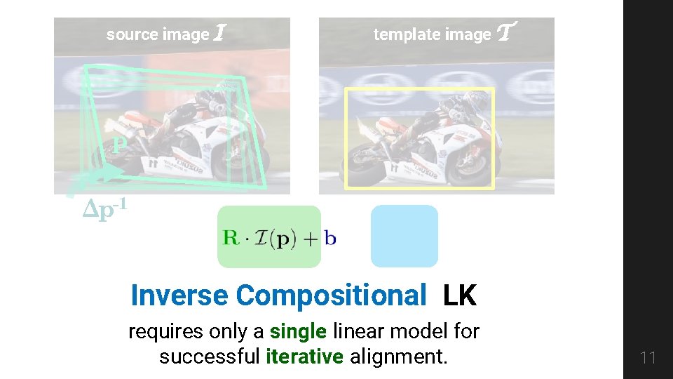
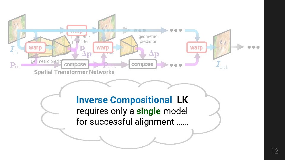
source image I template image T p Δp-1 Inverse Compositional LK requires only a single linear model for successful iterative alignment. 11

warp Iin pin geometric predictor p Δp warp … … warp I out pout compose Spatial Transformer Networks geometric predictor Δp compose … … … warp Iout Geometry effect is preserved 1. Boundary Allows iterative alignment (LK) 2. Single transformation Inverse Compositional LK requires only a single model for successful alignment …… 12

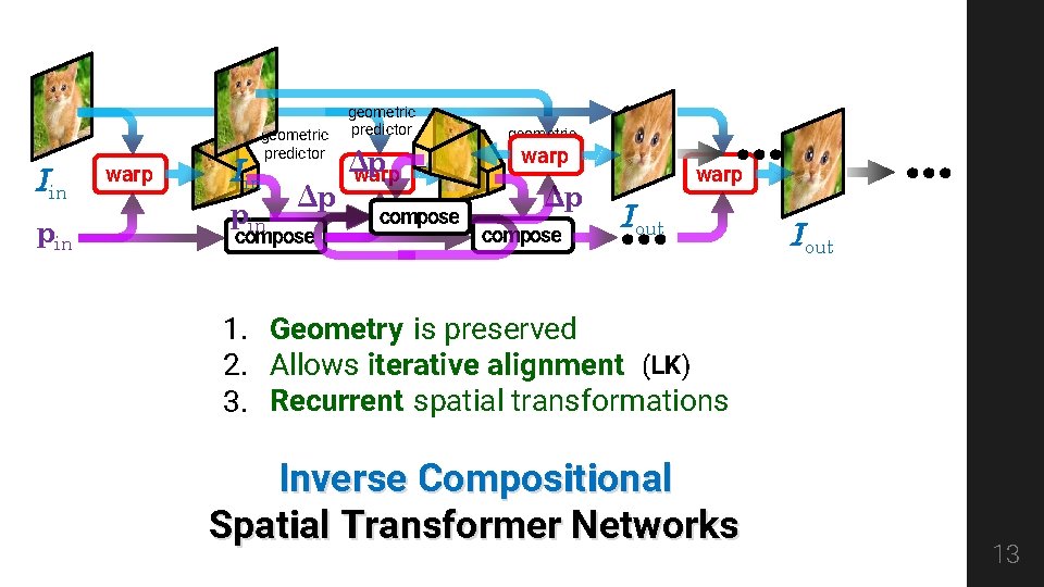
Iin pin warp geometric predictor Iin Δp pin compose geometric predictor Δp warp compose geometric predictor warp Δp compose … … warp Iout 1. Geometry is preserved 2. Allows iterative alignment (LK) 3. Recurrent spatial transformations Inverse Compositional Spatial Transformer Networks 13

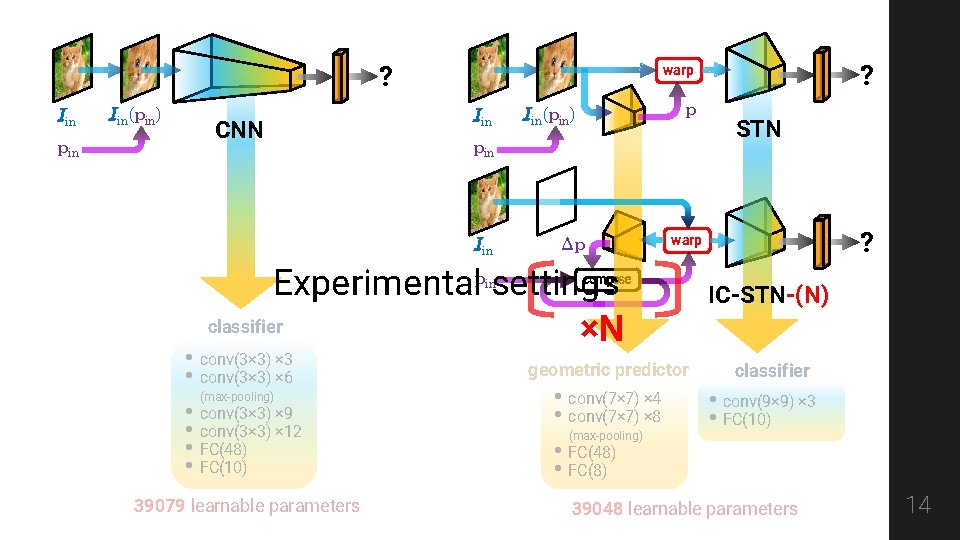
? Iin pin Iin(pin) CNN Iin p Iin(pin) pin Iin Δp in 39079 learnable parameters compose geometric predictor • conv(7× 7) × 4 • conv(7× 7) × 8 (max-pooling) • FC(48) • FC(8) STN ? warp Experimentalp settings classifier ×N • conv(3× 3) × 3 • conv(3× 3) × 6 (max-pooling) • conv(3× 3) × 9 • conv(3× 3) × 12 • FC(48) • FC(10) ? warp IC-STN-(N) classifier • conv(9× 9) × 3 • FC(10) 39048 learnable parameters 14

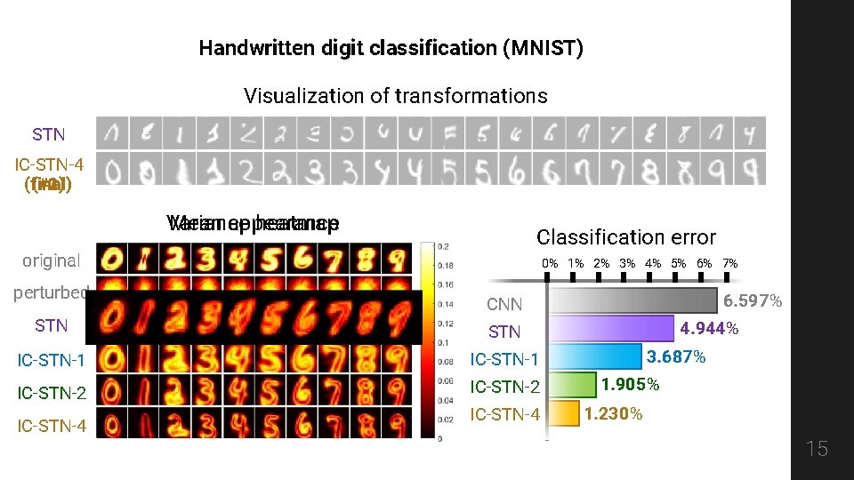
Handwritten digit classification (MNIST) Visualization of transformations STN IC-STN-4 (final) (#3) (#2) (#1) Variance Mean appearance heatmap Classification error original perturbed 0% 1% 2% 3% 4% 5% 6% 7% STN IC-STN-1 IC-STN-2 IC-STN-4 6. 597% CNN IC-STN-4 4. 944% 3. 687% 1. 905% 1. 230% 15

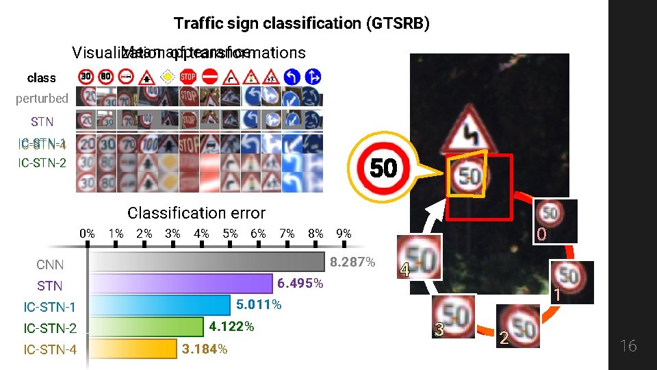
Traffic sign classification (GTSRB) Mean appearance Visualization of transformations class 30 80 perturbed STN IC-STN-1 IC-STN-4 IC-STN-2 50 Classification error 0% 1% 2% 3% 4% 5% 6% 7% 8% 8. 287% CNN 6. 495% STN IC-STN-4 4 1 5. 011% IC-STN-1 IC-STN-2 0 9% 4. 122% 3. 184% 3 2 16

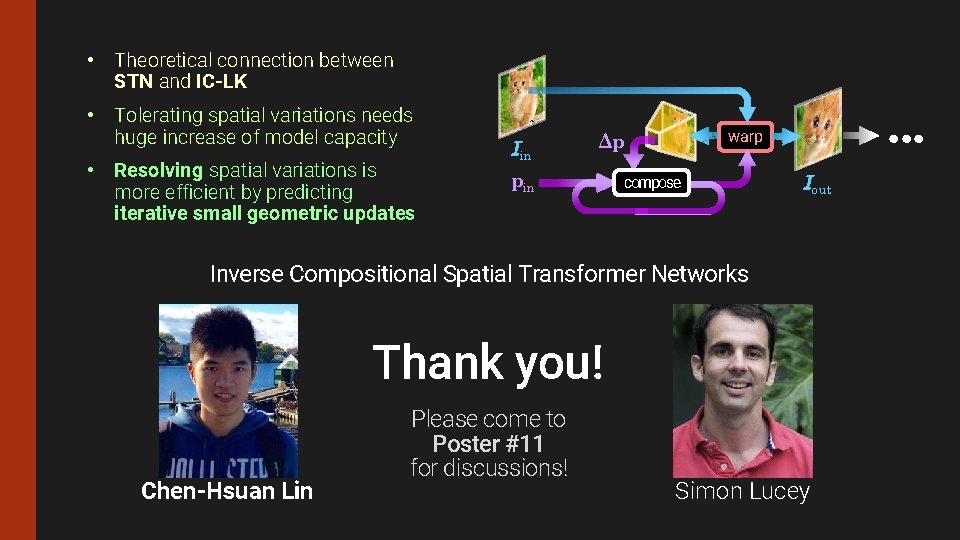
• Theoretical connection between STN and IC-LK • Tolerating spatial variations needs huge increase of model capacity • Resolving spatial variations is more efficient by predicting iterative small geometric updates Iin pin … warp Δp compose Iout Inverse Compositional Spatial Transformer Networks Thank you! Chen-Hsuan Lin Please come to Poster #11 for discussions! Simon Lucey