1 Starting Soon Geospatial Analysis for Optimization at

1 Starting Soon: Geospatial Analysis for Optimization at Environmental Sites (GRO-1) Guidance Document at http: //www. itrcweb. org/gro-1 Download Power. Point file • Clu-in training page at www. clu-in. org/conf/itrc/gro/ • Under “Download Training Materials” Using Adobe Connect • Full Screen button near top of page • Related Links (on right) § Select name of link § Click “Browse To” • Submit questions in the lower right

2 Welcome – Thanks for joining this ITRC Training Class Geospatial Analysis for Optimization at Environmental Sites (GRO-1) Guidance Document Sponsored by: Interstate Technology and Regulatory Council (www. itrcweb. org) Hosted by: US EPA Clean Up Information Network (www. cluin. org)

3 Housekeeping Course time is 2¼ hours This event is being recorded Trainers control slides • Want to control your own slides? You can download presentation file on Clu-in training page Questions and feedback • Throughout training: type in the “Q & A” box • At Q&A breaks: unmute your phone with #6 to ask out loud • At end of class: Feedback form available from last slide § Need confirmation of your participation today? Fill out the feedback form and check box for confirmation email and certificate Copyright 2018 Interstate Technology & Regulatory Council, 50 F Street, NW, Suite 350, Washington, DC 20001

4 ITRC (www. itrcweb. org) – Shaping the Future of Regulatory Acceptance Host organization Network • State regulators Disclaimer • Full version in “Notes” section • Partially funded by the U. S. government § All 50 states, PR, DC § ITRC nor US government • Federal partners warranty material § ITRC nor US government DOE DOD • ITRC Industry Affiliates Program • Academia • Community stakeholders Follow ITRC endorse specific products EPA ITRC materials available for your use – see usage policy Available from www. itrcweb. org • Technical and regulatory guidance documents • Online and classroom training schedule • More…

5 Meet the ITRC Trainers Dave Becker Chris Stubbs US Army Corps of Engineers Omaha, NE 402 -697 -2655 Dave. j. becker @usace. army. mil Ramboll Emeryville, CA 510 -420 -2552 cstubbs @ramboll. com Adam Janzen Barr Engineering Company Minneapolis, MN 952 -842 -3596 ajanzen@barr. com Ed Winner Kentucky Underground Storage Tank Branch Frankfort, KY 502 -564 -5981 Edward. Winner@ky. gov Read trainer bios at https: //clu-in. org/conf/itrc/GRO/

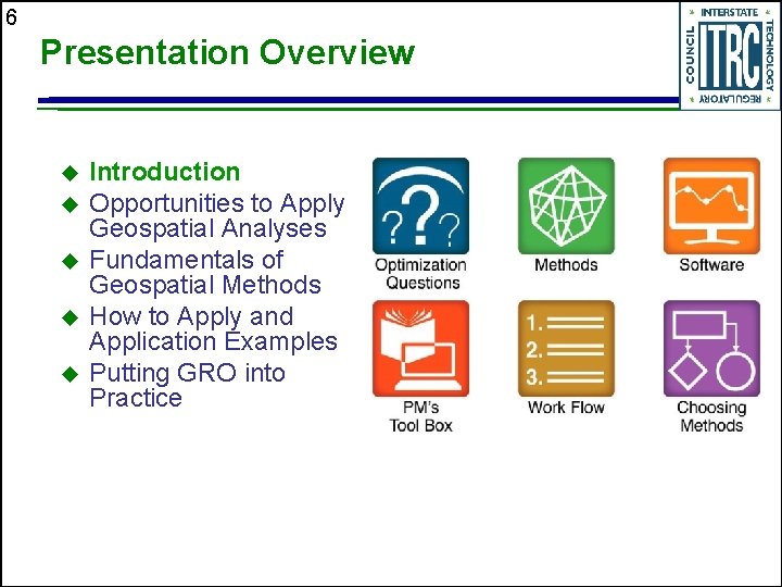
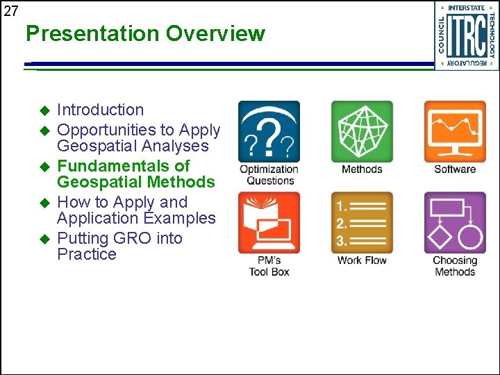
6 Presentation Overview Introduction Opportunities to Apply Geospatial Analyses Fundamentals of Geospatial Methods How to Apply and Application Examples Putting GRO into Practice

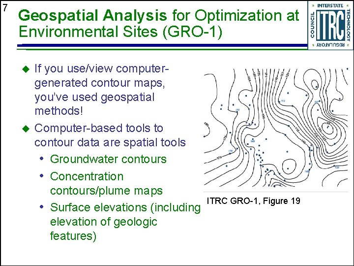
7 Geospatial Analysis for Optimization at Environmental Sites (GRO-1) If you use/view computergenerated contour maps, you’ve used geospatial methods! Computer-based tools to contour data are spatial tools • Groundwater contours • Concentration contours/plume maps • Surface elevations (including elevation of geologic features) ITRC GRO-1, Figure 19

8 Geospatial Analysis for Optimization at Environmental Sites (GRO-1) We are being asked to do more with less Agencies/Department of Defense have policies requiring optimization • Some focus on post construction • Others promote optimization throughout life cycle ITRC Remediation Process Optimization guidance documents and fact sheets Other tools • Federal Remediation Technology Roundtable (FRTR) • EPA Clu-in web sites have references, case studies • US Air Force tools ITRC GRO-1, History of Remedial Process Optimization

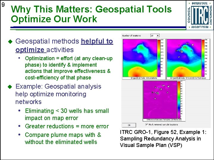
9 Why This Matters: Geospatial Tools Optimize Our Work Geospatial methods helpful to optimize activities • Optimization = effort (at any clean-up phase) to identify & implement actions that improve effectiveness & cost-efficiency of that phase Example: Geospatial analysis help optimize monitoring networks • Eliminating < 30 wells has small impact on map error • Greater reductions = more error • Compare plume maps with & without the eliminated wells ITRC GRO-1, Figure 52, Example 1: Sampling Redundancy Analysis in Visual Sample Plan (VSP)

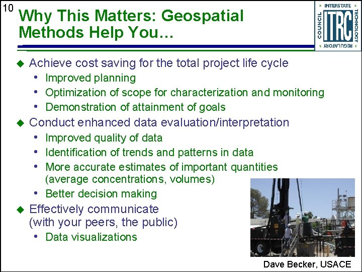
10 Why This Matters: Geospatial Methods Help You… Achieve cost saving for the total project life cycle • Improved planning • Optimization of scope for characterization and monitoring • Demonstration of attainment of goals Conduct enhanced data evaluation/interpretation • Improved quality of data • Identification of trends and patterns in data • More accurate estimates of important quantities (average concentrations, volumes) • Better decision making Effectively communicate (with your peers, the public) • Data visualizations Dave Becker, USACE

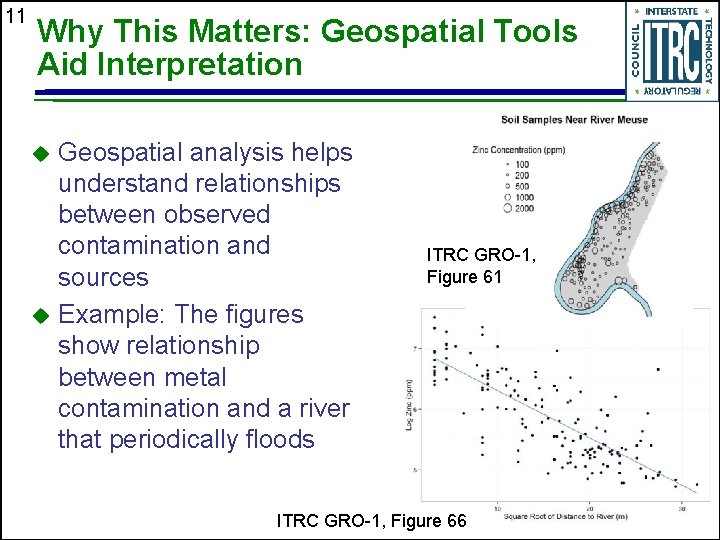
11 Why This Matters: Geospatial Tools Aid Interpretation Geospatial analysis helps understand relationships between observed contamination and sources Example: The figures show relationship between metal contamination and a river that periodically floods ITRC GRO-1, Figure 61 ITRC GRO-1, Figure 66

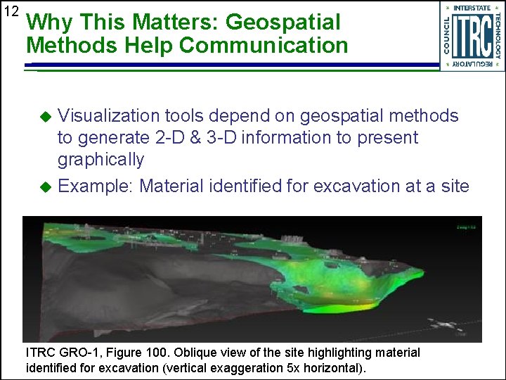
12 Why This Matters: Geospatial Methods Help Communication Visualization tools depend on geospatial methods to generate 2 -D & 3 -D information to present graphically Example: Material identified for excavation at a site ITRC GRO-1, Figure 100. Oblique view of the site highlighting material identified for excavation (vertical exaggeration 5 x horizontal).

13 Poll Question What role would you likely play in application of geospatial analysis? • Project manager overseeing team members who • • conduct the analysis Technical reviewer of geospatial analysis Technical practitioner applying the methods Stakeholder interested in understanding basis and meaning of the results of geospatial analyses Others

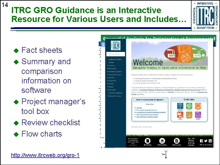
14 ITRC GRO Guidance is an Interactive Resource for Various Users and Includes… Fact sheets Summary and comparison information on software Project manager’s tool box Review checklist Flow charts http: //www. itrcweb. org/gro-1

15 Training and Guidance Objectives: Learning objectives: With the ITRC Geospatial Analysis for Optimization guidance document and this associated training, project managers/technical staff will be able to: Determine if appropriate - based on available data & site needs, determine if geospatial analyses are appropriate for site Identify questions - for project and specific lifecycle stage, identify optimization questions to ask Select method(s) - select appropriate geospatial method(s) and software to answer questions Explain and apply results - explain what the results mean and appropriately apply in decision making NOTE! Training is meant primarily to give you a taste of the critical concepts and provide overview of the guidance.

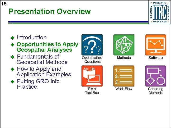
16 Presentation Overview Introduction Opportunities to Apply Geospatial Analyses Fundamentals of Geospatial Methods How to Apply and Application Examples Putting GRO into Practice

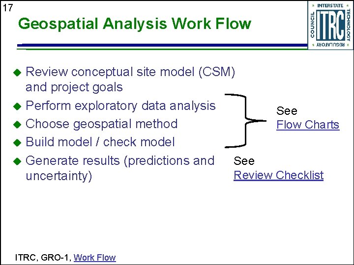
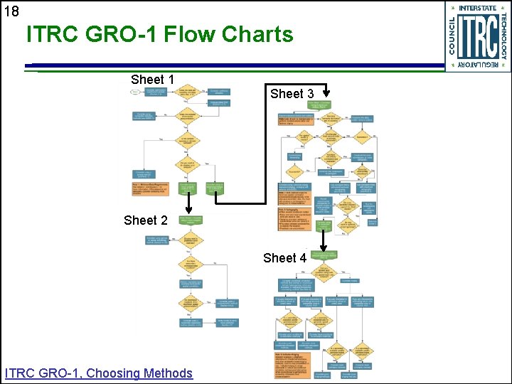
17 Geospatial Analysis Work Flow Review conceptual site model (CSM) and project goals Perform exploratory data analysis See Choose geospatial method Flow Charts Build model / check model Generate results (predictions and See Review Checklist uncertainty) ITRC, GRO-1, Work Flow

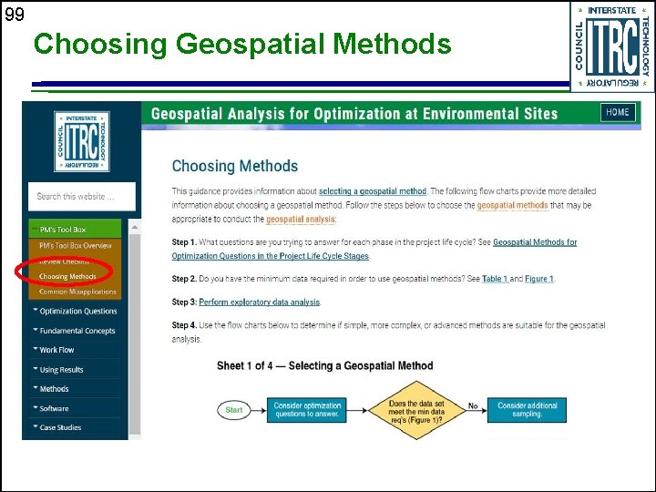
18 ITRC GRO-1 Flow Charts Sheet 1 Sheet 3 Sheet 2 Sheet 4 ITRC GRO-1, Choosing Methods

19 Applications of Geospatial Methods What are the data requirements? Regulatory barriers and concerns – Fact Sheet 1 What are the common misapplications? Using geospatial methods to support optimization • Optimization questions one may ask at various project phases for which geospatial methods can be used

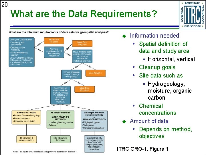
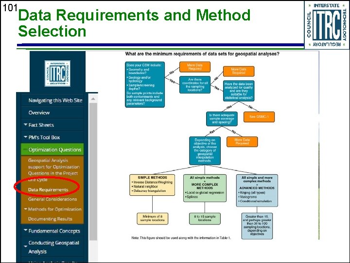
20 What are the Data Requirements? Information needed: • Spatial definition of data and study area § Horizontal, vertical • Cleanup goals • Site data such as § Hydrogeology, moisture, organic carbon • Chemical concentrations Amount of data • Depends on method, objectives ITRC GRO-1, Figure 1

21 Regulatory Barriers and Concerns Many state and federal agencies have accepted approaches for optimization Guidelines vary by agency – user should identify before proceeding Modification of project life-cycle activities can be difficult from a regulatory perspective Hesitance to use or accept new geospatial analysis POLL QUESTION: Have you experienced resistance to using geospatial methods for a project?

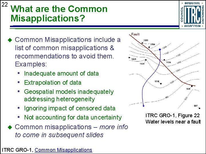
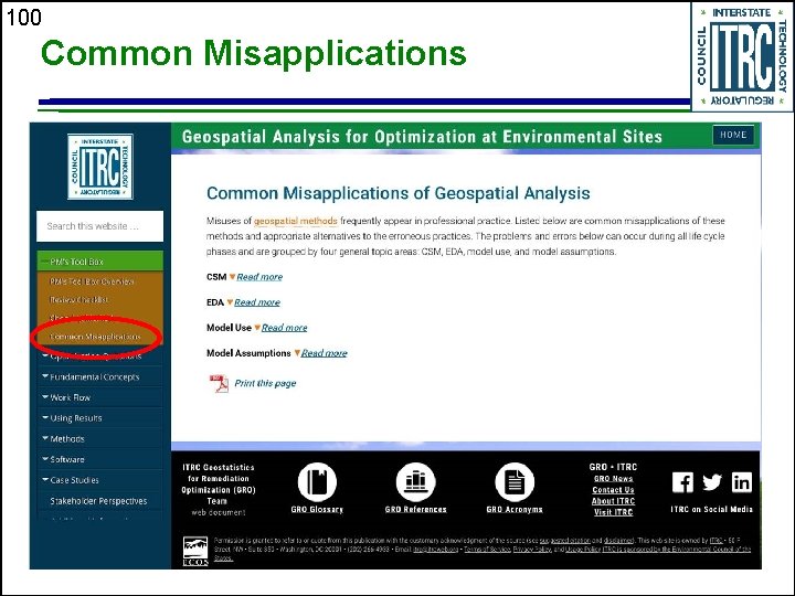
22 What are the Common Misapplications? Common Misapplications include a list of common misapplications & recommendations to avoid them. Examples: • Inadequate amount of data • Extrapolation of data • Geospatial models inadequately addressing heterogeneity • Ignoring impact of censored data • Not accounting for data uncertainty Common misapplications – more info to come in subsequent slides ITRC GRO-1, Common Misapplications ITRC GRO-1, Figure 22 Water levels near a fault

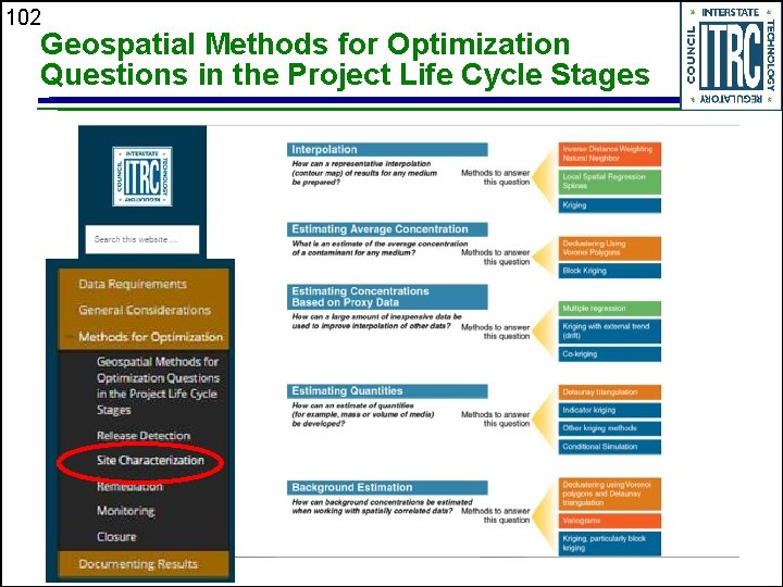
23 Optimization Questions – Examples for Different Project Phases Release Detection: • Do the detected concentrations represent an actual plume? • Note there is often only spatially sparse data at this phase Site Characterization: • What is appropriate sample spacing, considering spatial correlation? Remediation: • What are the estimated average concentrations (for treatment design)? ITRC GRO-1, Optimization Questions Monitoring • How can geospatial methods help optimize a monitoring program? Closure • Can geospatial methods help determine if the monitoring program is adequate for closure? • Note that spatial data are often sparse near closure Dave Becker, USACE

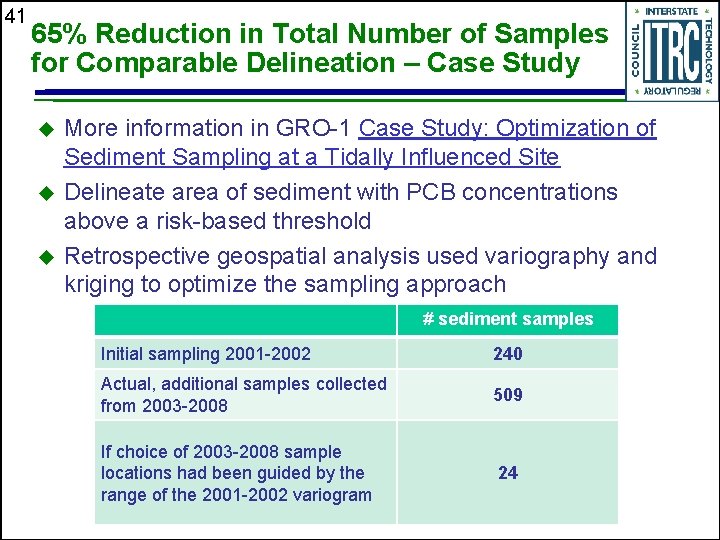
24 Example of Life-Cycle Optimization Question & Geospatial Methods to Apply Site characterization phase – “What is appropriate sample spacing, considering spatial correlation? ” • Planning for cost-effective sampling: choosing sampling spacing to characterize soil contamination • Use geospatial analyses to estimate sample spacing to avoid duplication of information (spatial correlation) • Construct variogram (will be discussed in more detail), determine geostatistical range, use as basis for sample spacing with independent data • Software to do this can be located using guidance ITRC GRO-1, Site Characterization

25 Where to Next? Answering the Questions Geospatial methods are identified that may answer these questions and are generally categorized into: • Simple • More complex • Advanced Software tools are identified to apply the proposed methods

26 Poll Question Based on what we’ve presented in this section, do you work on sites that could benefit from geospatial analysis? • • Yes No, not enough data No, we don’t need geospatial analysis Don’t know yet

27 Presentation Overview Introduction Opportunities to Apply Geospatial Analyses Fundamentals of Geospatial Methods How to Apply and Application Examples Putting GRO into Practice

28 After Fundamentals Section, You Can… Explain how geospatial methods work • Classification and components • Variograms – key concept for geospatial analysis Avoid misapplications

29 Basic Premise of Geospatial Methods Tobler’s First Law of Geography (Tobler 1970): “Everything is related to everything else, but near things are more related than distant things. ” Sample observations collected close together in space or time are more related than sample observations collected farther apart. This is the basic premise of geospatial methods ITRC GRO-1, Fundamental Concepts

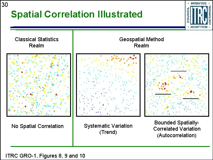
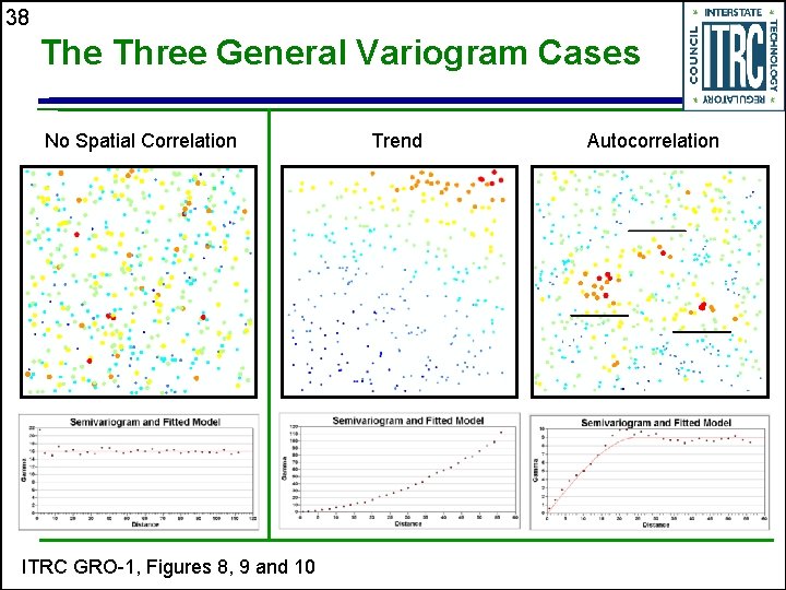
30 Spatial Correlation Illustrated Classical Statistics Realm No Spatial Correlation Geospatial Method Realm Systematic Variation (Trend) ITRC GRO-1, Figures 8, 9 and 10 Bounded Spatially. Correlated Variation (Autocorrelation)

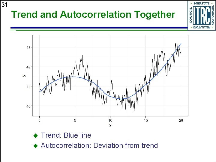
31 Trend and Autocorrelation Together Trend: Blue line Autocorrelation: Deviation from trend

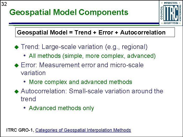
32 Geospatial Model Components Geospatial Model = Trend + Error + Autocorrelation Trend: Large-scale variation (e. g. , regional) • All methods (simple, more complex, advanced) Error: Measurement error and micro-scale variation • More complex and advanced methods Autocorrelation: Small-scale variation around the trend • Advanced methods only ITRC GRO-1, Categories of Geospatial Interpolation Methods

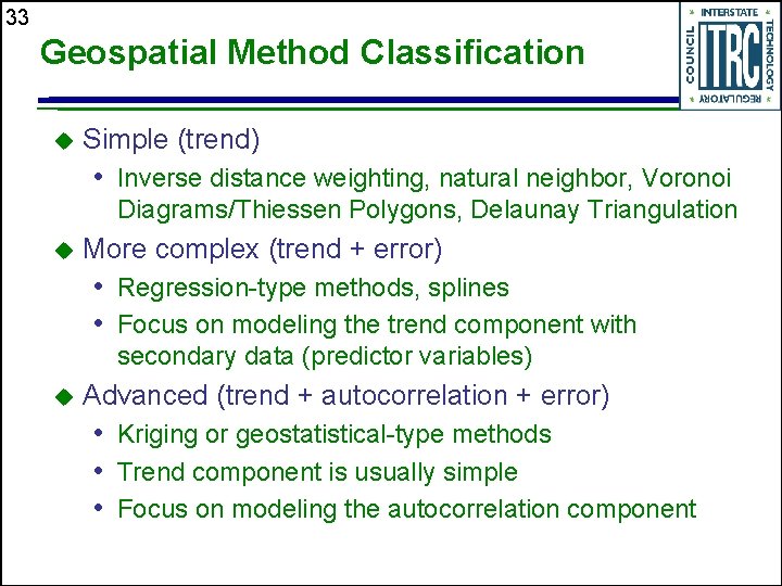
33 Geospatial Method Classification Simple (trend) • Inverse distance weighting, natural neighbor, Voronoi Diagrams/Thiessen Polygons, Delaunay Triangulation More complex (trend + error) • Regression-type methods, splines • Focus on modeling the trend component with secondary data (predictor variables) Advanced (trend + autocorrelation + error) • Kriging or geostatistical-type methods • Trend component is usually simple • Focus on modeling the autocorrelation component

34 Simple Methods for Maps, More Complex or Advanced for Optimization Simple methods focus on making good maps • “Good” is typically evaluated visually • Map should be consistent with CSM Many optimization tasks require more than just mapping. • More complex and advanced methods are based on statistical modeling • They produce more accurate predictions with estimates of uncertainty More complex and advanced methods can also be “simple” methods when using default parameters. This is acceptable for mapping ONLY.

35 Why Is Spatial Correlation Important? Good news: spatial correlation allows mapping between samples! • Used by all methods to interpolate between sample locations Bad news: correlated samples reduce uncertainty less than independent samples • Need to understand correlation scale to optimize sampling • Sample spacing << correlation scale do not provide much additional information

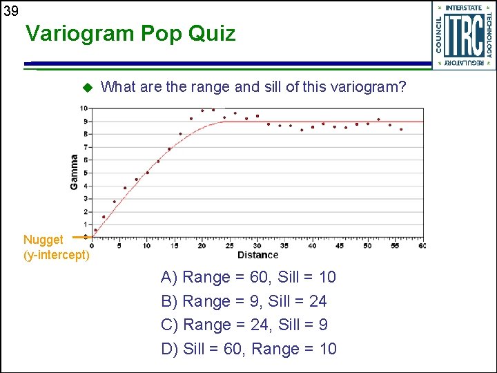
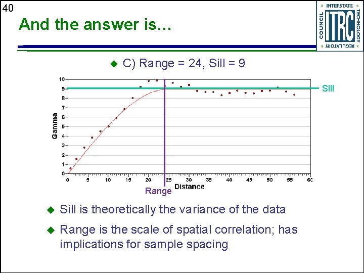
36 Quantifying Spatial Correlation with Variograms The variogram (or semivariogram) quantifies spatial correlation The variogram is a plot of the squared differences between measured values as a function of distance between sampling locations Kriging requires a variogram (autocorrelation model) Variogram is also useful by itself to identify the scale of spatial correlation

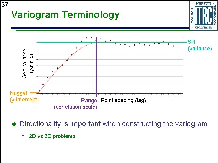
37 Variogram Terminology Semivariance (gamma) Sill (variance) Nugget (y-intercept) Range Point spacing (lag) (correlation scale) Directionality is important when constructing the variogram • 2 D vs 3 D problems

38 The Three General Variogram Cases No Spatial Correlation ITRC GRO-1, Figures 8, 9 and 10 Trend Autocorrelation

39 Variogram Pop Quiz What are the range and sill of this variogram? Nugget (y-intercept) A) Range = 60, Sill = 10 B) Range = 9, Sill = 24 C) Range = 24, Sill = 9 D) Sill = 60, Range = 10

40 And the answer is… C) Range = 24, Sill = 9 Sill Range Sill is theoretically the variance of the data Range is the scale of spatial correlation; has implications for sample spacing

41 65% Reduction in Total Number of Samples for Comparable Delineation – Case Study More information in GRO-1 Case Study: Optimization of Sediment Sampling at a Tidally Influenced Site Delineate area of sediment with PCB concentrations above a risk-based threshold Retrospective geospatial analysis used variography and kriging to optimize the sampling approach # sediment samples Initial sampling 2001 -2002 240 Actual, additional samples collected from 2003 -2008 509 If choice of 2003 -2008 sample locations had been guided by the range of the 2001 -2002 variogram 24

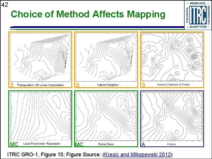
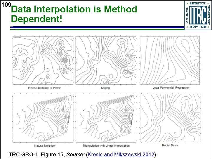
42 Choice of Method Affects Mapping S S S MC MC A ITRC GRO-1, Figure 15; Figure Source: (Kresic and Mikszewski 2012)

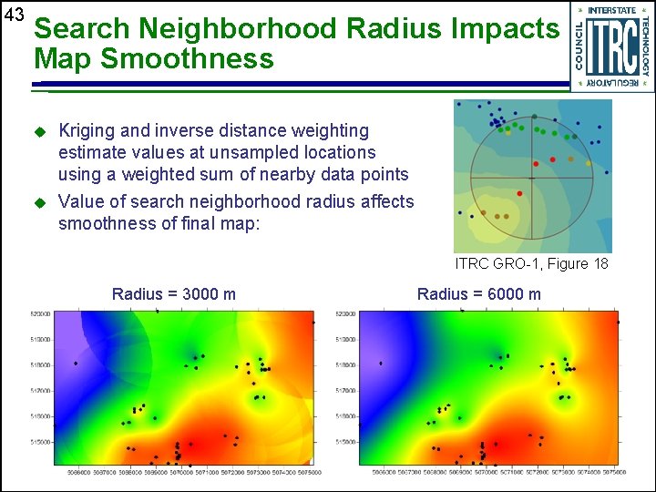
43 Search Neighborhood Radius Impacts Map Smoothness Kriging and inverse distance weighting estimate values at unsampled locations using a weighted sum of nearby data points Value of search neighborhood radius affects smoothness of final map: ITRC GRO-1, Figure 18 Radius = 3000 m Radius = 6000 m

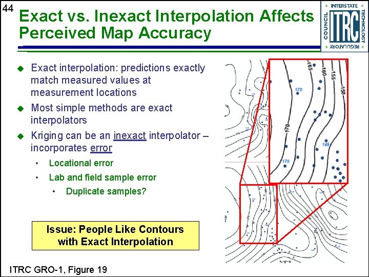
44 Exact vs. Inexact Interpolation Affects Perceived Map Accuracy Exact interpolation: predictions exactly match measured values at measurement locations Most simple methods are exact interpolators Kriging can be an inexact interpolator – incorporates error • Locational error • Lab and field sample error • Duplicate samples? Issue: People Like Contours with Exact Interpolation ITRC GRO-1, Figure 19

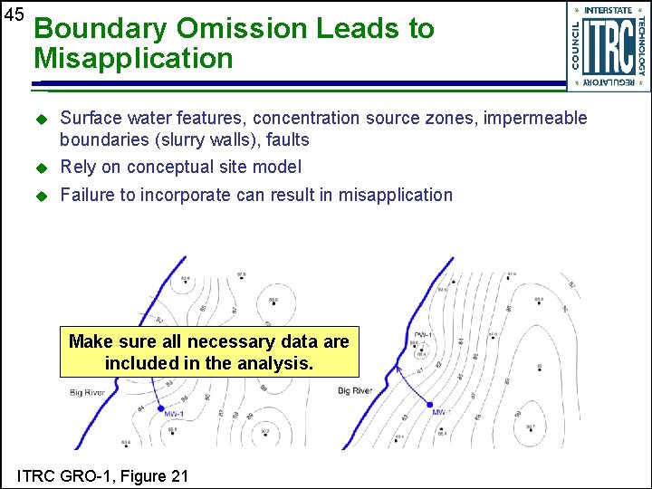
45 Boundary Omission Leads to Misapplication Surface water features, concentration source zones, impermeable boundaries (slurry walls), faults Rely on conceptual site model Failure to incorporate can result in misapplication Make sure all necessary data are included in the analysis. ITRC GRO-1, Figure 21

46 Fundamentals Section Wrap Up Data must show spatial correlation in order to use geospatial methods Geospatial model = Trend + Error + Autocorrelation Variograms quantify spatial correlation and are a key concept in geospatial analysis Choose a geospatial method consistent with your CSM

47 Question & Answer Break

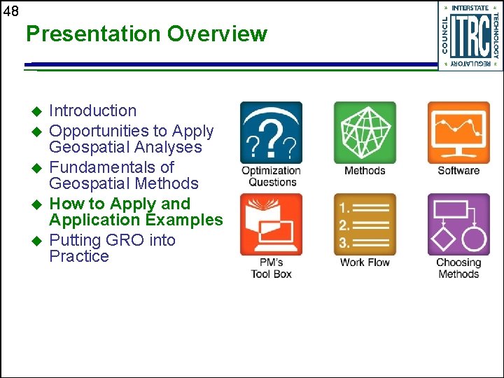
48 Presentation Overview Introduction Opportunities to Apply Geospatial Analyses Fundamentals of Geospatial Methods How to Apply and Application Examples Putting GRO into Practice

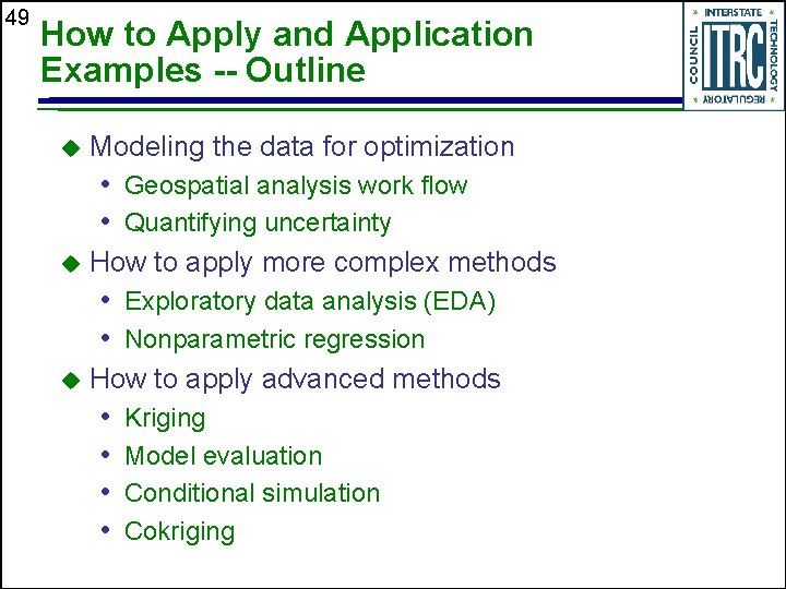
49 How to Apply and Application Examples -- Outline Modeling the data for optimization • Geospatial analysis work flow • Quantifying uncertainty How to apply more complex methods • Exploratory data analysis (EDA) • Nonparametric regression How to apply advanced methods • • Kriging Model evaluation Conditional simulation Cokriging

50 Modeling the Data for Optimization Quantitative predictions for optimization require modeling the data with more complex or advanced methods • Predictions are more accurate • Uncertainty in predictions can be quantified • Sampling can be better optimized Modeling goes beyond mapping the data • Fit statistical model to the data • Assess accuracy of predictions ITRC GRO-1, More Complex Methods, Advanced Methods

51 Follow the Geospatial Work Flow Practitioners • Conduct the geospatial analysis • Follow the work flow to model the data • Document each step of work flow Reviewers • Review the geospatial analysis • Follow the work flow to check that model is appropriate • Verify that documentation includes each step of work flow

52 Geospatial Analysis Work Flow Review CSM and project goals • Identify key site features and questions Perform exploratory data analysis • Evaluate distribution, outliers, trend, spatial correlation, auxiliary data Choose geospatial method • Simple, more complex, advanced Build model / check model • Cross-validation and CSM consistency Generate results (predictions and uncertainty) ITRC GRO-1, Work Flow Overview

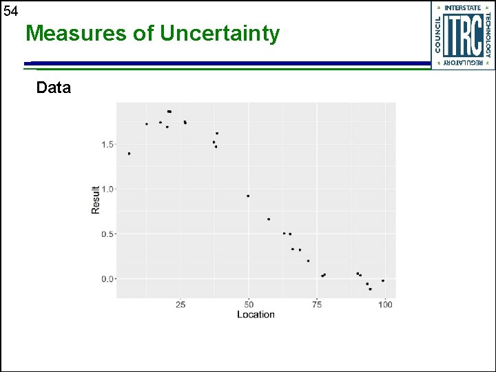
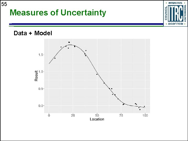
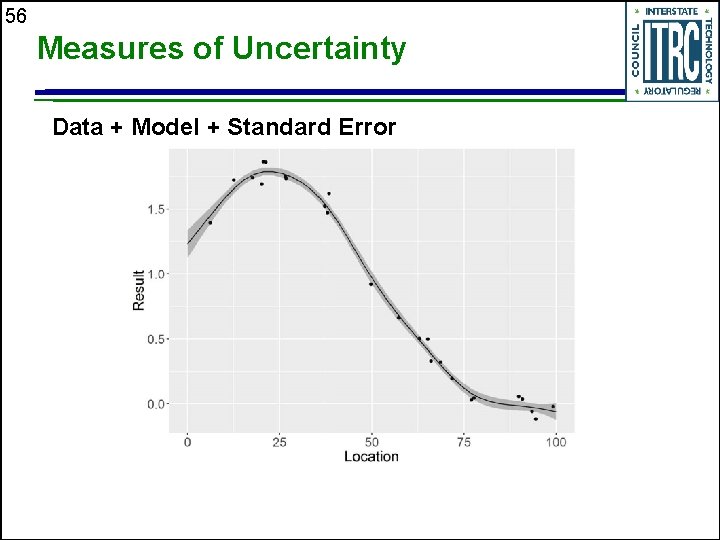
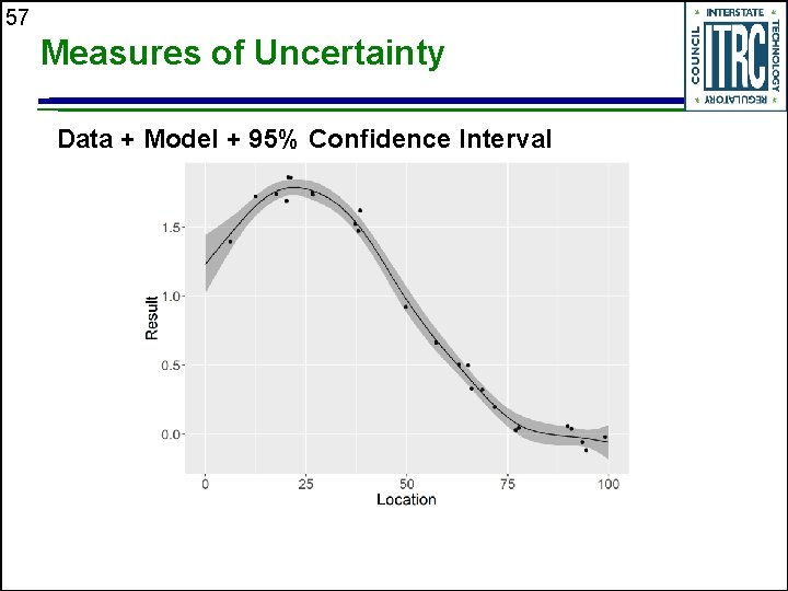
53 Measures of Uncertainty Standard error and variance • Output of more complex and advanced methods Confidence/prediction interval • Can be calculated from predictions and standard error or variance Exceedance probability • Probability of exceeding a threshold ITRC GRO-1, Evaluate Accuracy, Generate Results

54 Measures of Uncertainty Data

55 Measures of Uncertainty Data + Model

56 Measures of Uncertainty Data + Model + Standard Error

57 Measures of Uncertainty Data + Model + 95% Confidence Interval

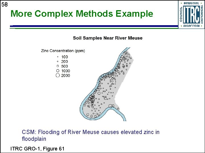
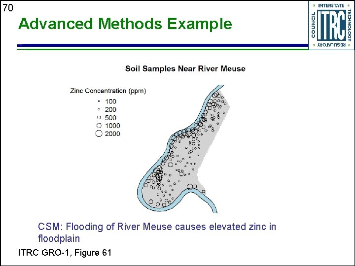
58 More Complex Methods Example CSM: Flooding of River Meuse causes elevated zinc in floodplain ITRC GRO-1, Figure 61

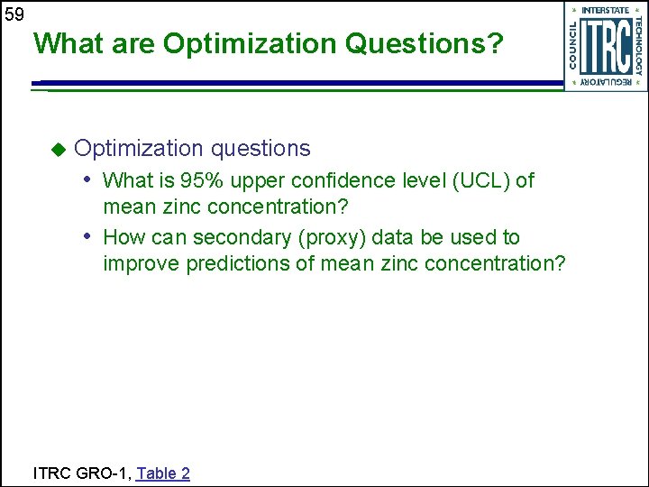
59 What are Optimization Questions? Optimization questions • What is 95% upper confidence level (UCL) of mean zinc concentration? • How can secondary (proxy) data be used to improve predictions of mean zinc concentration? ITRC GRO-1, Table 2

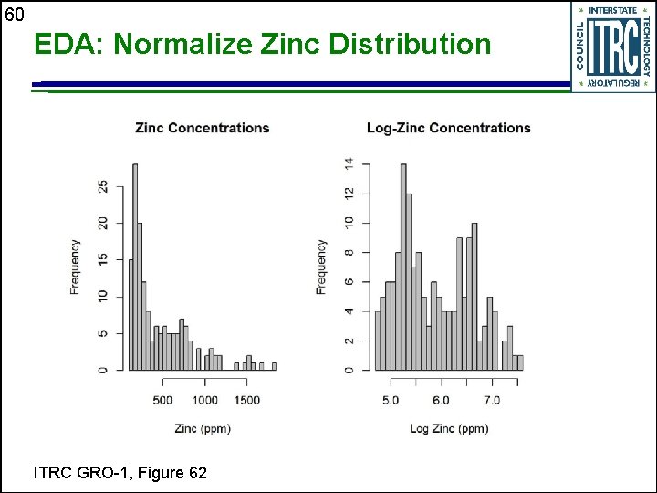
60 EDA: Normalize Zinc Distribution ITRC GRO-1, Figure 62

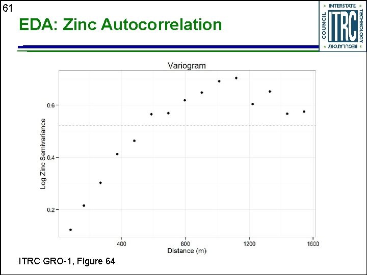
61 EDA: Zinc Autocorrelation ITRC GRO-1, Figure 64

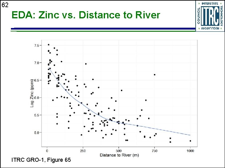
62 EDA: Zinc vs. Distance to River ITRC GRO-1, Figure 65

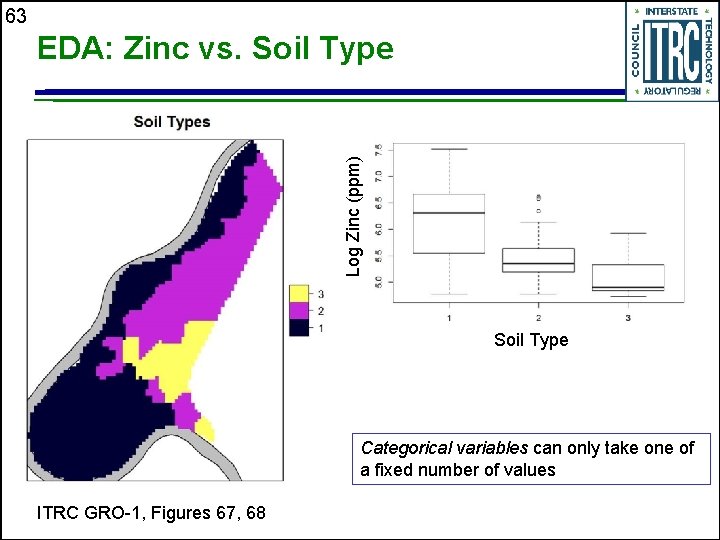
63 Log Zinc (ppm) EDA: Zinc vs. Soil Type Categorical variables can only take one of a fixed number of values ITRC GRO-1, Figures 67, 68

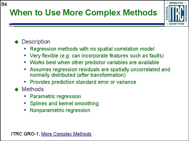
64 When to Use More Complex Methods Description • • Regression methods with no spatial correlation model Very flexible (e. g. can incorporate features such as faults) Works best when other predictor variables are available Assumes regression residuals are spatially uncorrelated and normally distributed (after transformation) • Provides prediction standard error or variance Methods • Parametric regression • Splines and kernel smoothing • Nonparametric regression ITRC GRO-1, More Complex Methods

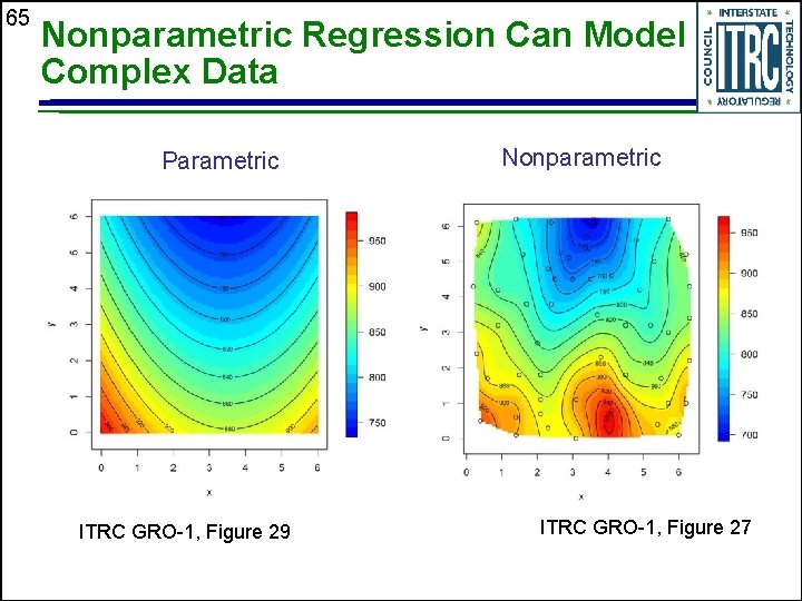
65 Nonparametric Regression Can Model Complex Data Parametric ITRC GRO-1, Figure 29 Nonparametric ITRC GRO-1, Figure 27

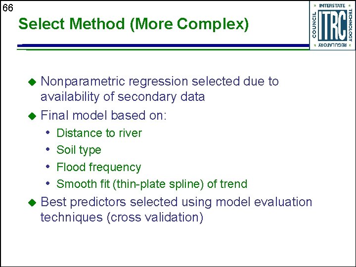
66 Select Method (More Complex) Nonparametric regression selected due to availability of secondary data Final model based on: • • Distance to river Soil type Flood frequency Smooth fit (thin-plate spline) of trend Best predictors selected using model evaluation techniques (cross validation)

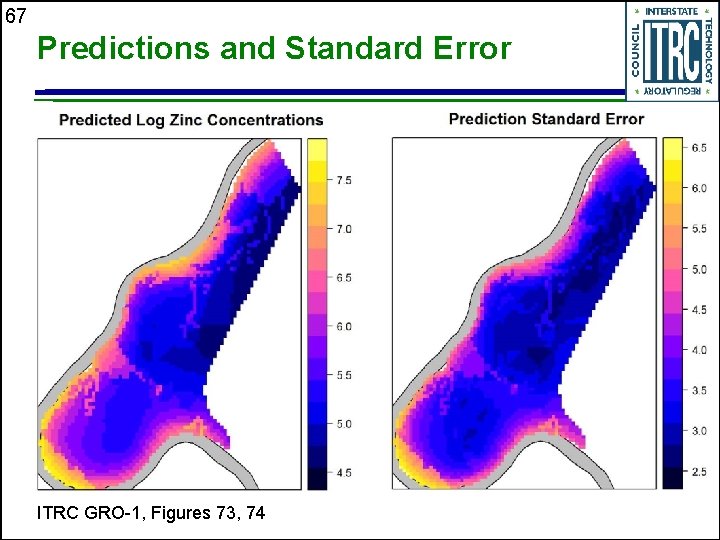
67 Predictions and Standard Error ITRC GRO-1, Figures 73, 74

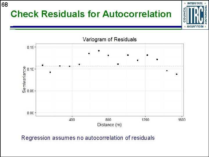
68 Check Residuals for Autocorrelation Regression assumes no autocorrelation of residuals

69 Use Model for Optimization Calculate average concentration with confidence limits to compare to remediation target concentration Optimize sampling/remediation • Locate additional samples at locations with highest uncertainty • Select subareas to target for remediation in order to reduce upper confidence limit below remediation target ITRC GRO-1, Using Results

70 Advanced Methods Example CSM: Flooding of River Meuse causes elevated zinc in floodplain ITRC GRO-1, Figure 61

71 Advanced Methods Example Same CSM and zinc data as Example 1, but no secondary data available Optimization questions • What is the area requiring remediation? • Where should additional samples be located? ITRC GRO-1, Table 2

72 When to Apply Advanced Methods Description • Extension of regression methods including a spatial correlation model • Works best when sufficient data to estimate correlation model are available • Assumes residuals after trend removal are stationary and normally distributed (after transformation) • Provides prediction standard error or variance Methods • Kriging/Cokriging (point and block) • Conditional simulation ITRC GRO-1, Advanced Methods

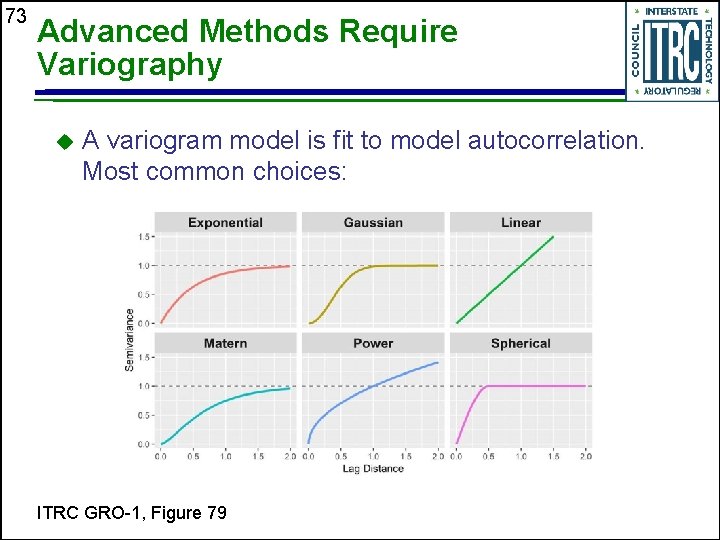
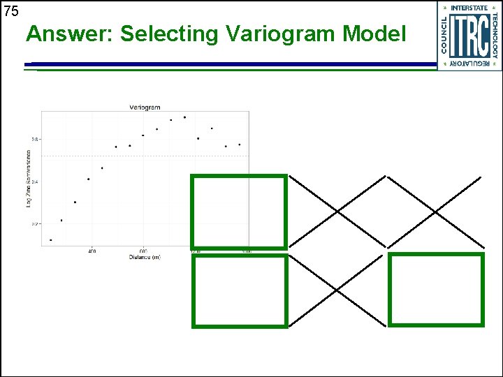
73 Advanced Methods Require Variography A variogram model is fit to model autocorrelation. Most common choices: ITRC GRO-1, Figure 79

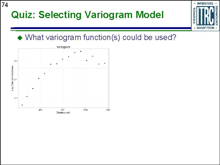
74 Quiz: Selecting Variogram Model What variogram function(s) could be used?

75 Answer: Selecting Variogram Model

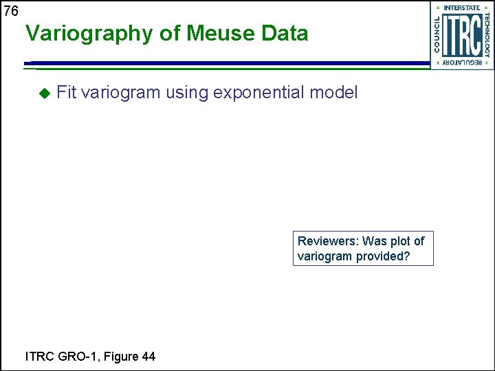
76 Variography of Meuse Data Fit variogram using exponential model Reviewers: Was plot of variogram provided? ITRC GRO-1, Figure 44

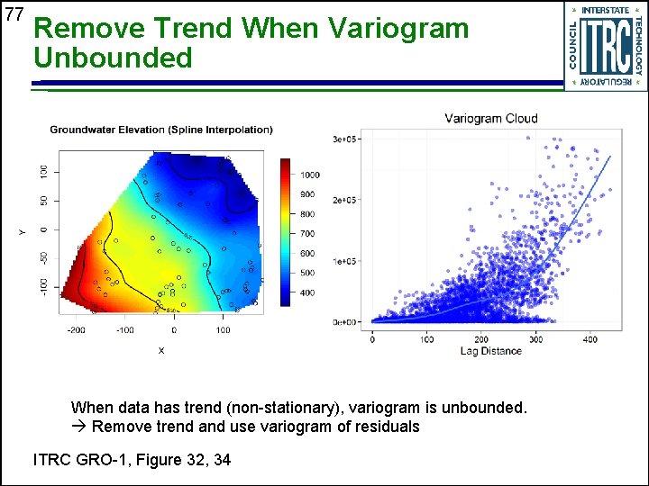
77 Remove Trend When Variogram Unbounded When data has trend (non-stationary), variogram is unbounded. Remove trend and use variogram of residuals ITRC GRO-1, Figure 32, 34

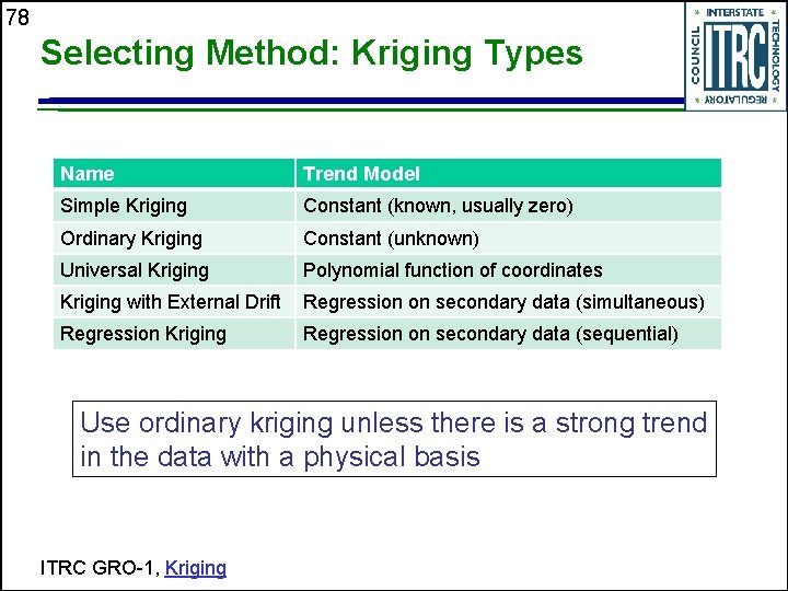
78 Selecting Method: Kriging Types Name Trend Model Simple Kriging Constant (known, usually zero) Ordinary Kriging Constant (unknown) Universal Kriging Polynomial function of coordinates Kriging with External Drift Regression on secondary data (simultaneous) Regression Kriging Regression on secondary data (sequential) Use ordinary kriging unless there is a strong trend in the data with a physical basis ITRC GRO-1, Kriging

79 Kriging of Zinc Concentration Ordinary Kriging (Spherical Variogram) Ordinary Kriging (Exponential Variogram)

80 Model Evaluation Evaluate consistency of predictions with CSM Verify assumptions of method Use cross-validation to quantitatively evaluate model quality • Can be used with any method • Take one out cross validation is most common • Look at accuracy of predictions and accuracy of prediction standard errors ITRC GRO-1, Evaluate Accuracy

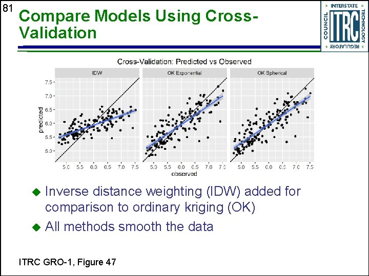
81 Compare Models Using Cross. Validation Inverse distance weighting (IDW) added for comparison to ordinary kriging (OK) All methods smooth the data ITRC GRO-1, Figure 47

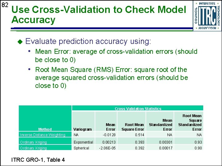
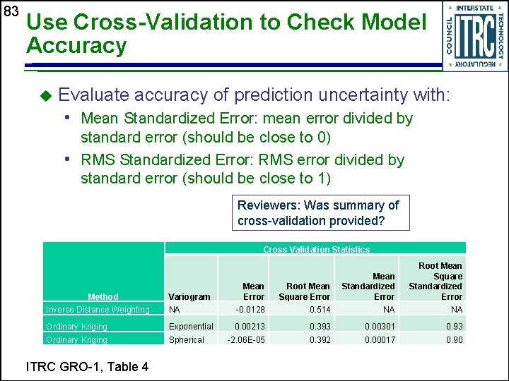
82 Use Cross-Validation to Check Model Accuracy Evaluate prediction accuracy using: • Mean Error: average of cross-validation errors (should be close to 0) • Root Mean Square (RMS) Error: square root of the average squared cross-validation errors (should be close to 0) Cross Validation Statistics Method Variogram Mean Error Root Mean Square Error Mean Standardized Error Root Mean Square Standardized Error Inverse Distance Weighting NA -0. 0128 0. 514 NA NA Ordinary Kriging Exponential 0. 00213 0. 393 0. 00301 0. 93 Ordinary Kriging Spherical -2. 06 E-05 0. 392 0. 00017 0. 90 ITRC GRO-1, Table 4

83 Use Cross-Validation to Check Model Accuracy Evaluate accuracy of prediction uncertainty with: • Mean Standardized Error: mean error divided by standard error (should be close to 0) • RMS Standardized Error: RMS error divided by standard error (should be close to 1) Reviewers: Was summary of cross-validation provided? Cross Validation Statistics Method Variogram Mean Error Root Mean Square Error Mean Standardized Error Root Mean Square Standardized Error Inverse Distance Weighting NA -0. 0128 0. 514 NA NA Ordinary Kriging Exponential 0. 00213 0. 393 0. 00301 0. 93 Ordinary Kriging Spherical -2. 06 E-05 0. 392 0. 00017 0. 90 ITRC GRO-1, Table 4

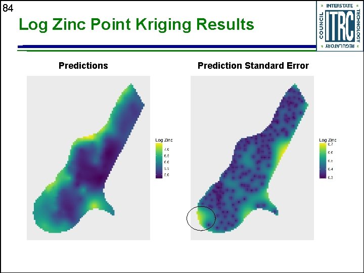
84 Log Zinc Point Kriging Results Prediction Standard Error

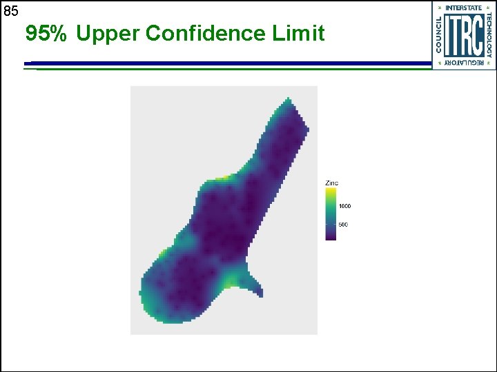
85 95% Upper Confidence Limit

86 Log Zinc Block Kriging Results Prediction Standard Error

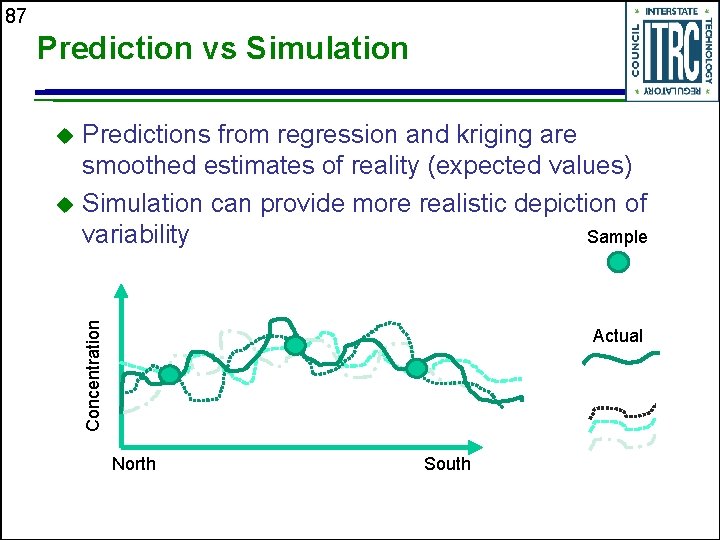
87 Prediction vs Simulation Predictions from regression and kriging are smoothed estimates of reality (expected values) Simulation can provide more realistic depiction of variability Sample Concentration Actual North South

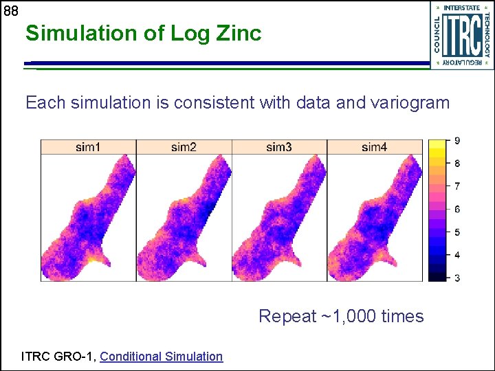
88 Simulation of Log Zinc Each simulation is consistent with data and variogram Repeat ~1, 000 times ITRC GRO-1, Conditional Simulation

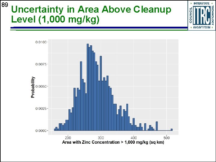
89 Uncertainty in Area Above Cleanup Level (1, 000 mg/kg)

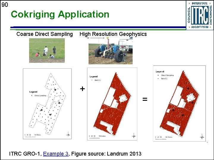
90 Cokriging Application Coarse Direct Sampling High Resolution Geophysics + = ITRC GRO-1, Example 3, Figure source: Landrum 2013

91 More Complex/Advanced Methods: Questions for Reviewers Is the method selected clearly described, along with a description of how it was implemented? Why was this method selected over alternative methods? Are the assumptions of the method met? How were the method parameters fit, and how was goodness-of-fit evaluated? Was prediction uncertainty described and quantified using cross-validation? Are the results consistent with the CSM? ITRC GRO-1, Review Checklist

92 Presentation Overview Introduction Opportunities to Apply Geospatial Analyses Fundamentals of Geospatial Methods How to Apply and Application Examples Putting GRO into Practice

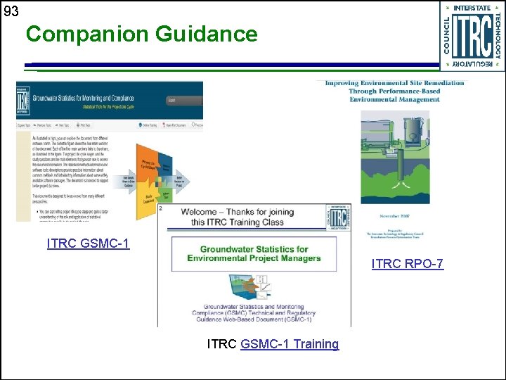
93 Companion Guidance ITRC GSMC-1 ITRC RPO-7 ITRC GSMC-1 Training

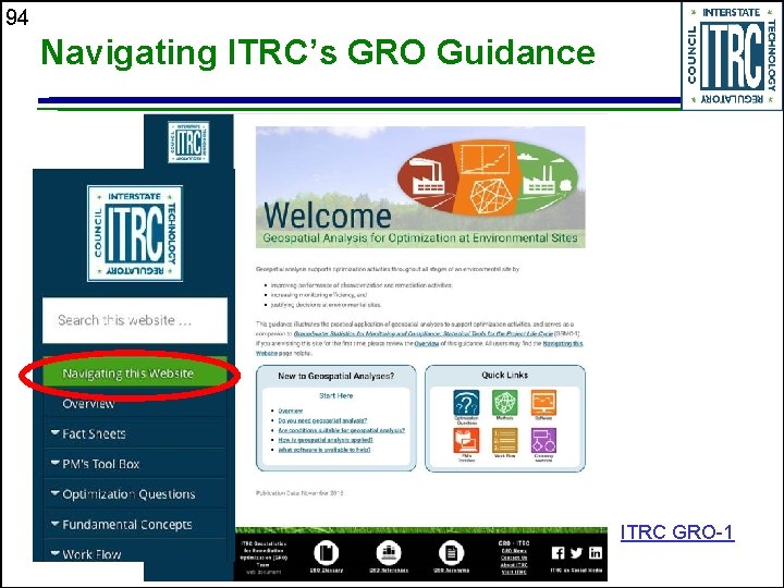
94 Navigating ITRC’s GRO Guidance ITRC GRO-1

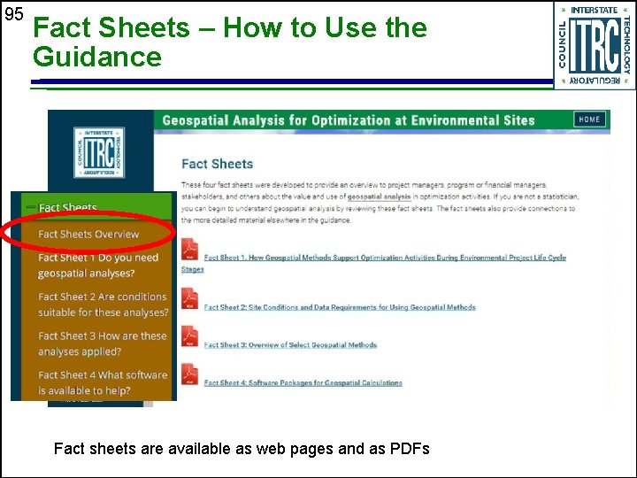
95 Fact Sheets – How to Use the Guidance Fact sheets are available as web pages and as PDFs

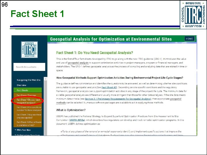
96 Fact Sheet 1

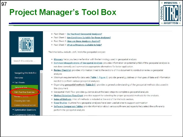
97 Project Manager’s Tool Box

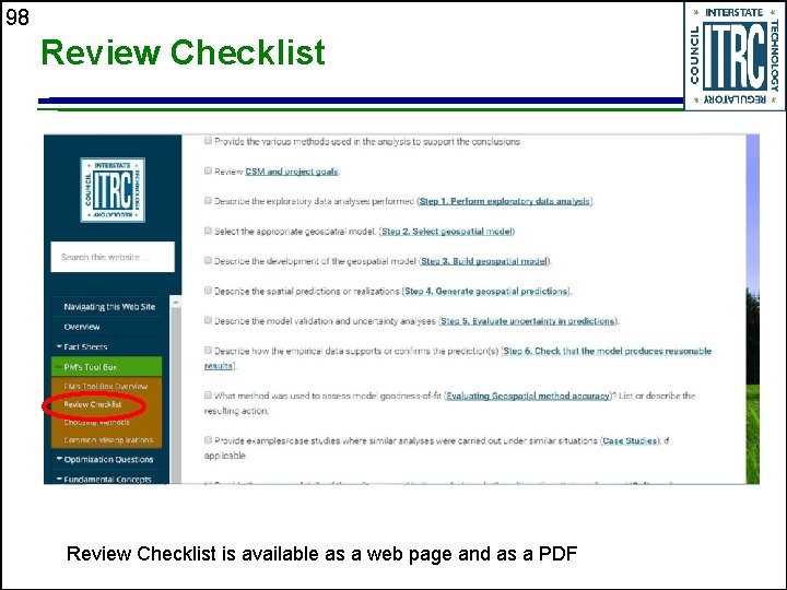
98 Review Checklist is available as a web page and as a PDF

99 Choosing Geospatial Methods

100 Common Misapplications

101 Data Requirements and Method Selection

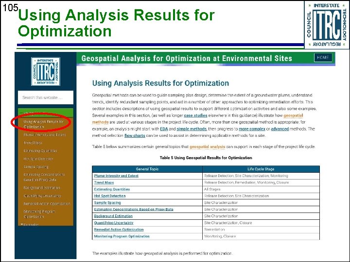
102 Geospatial Methods for Optimization Questions in the Project Life Cycle Stages

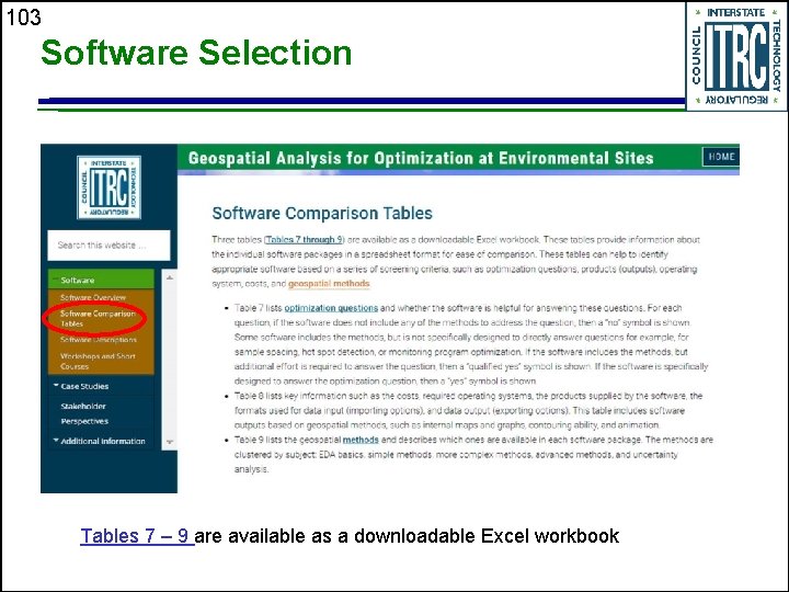
103 Software Selection Tables 7 – 9 are available as a downloadable Excel workbook

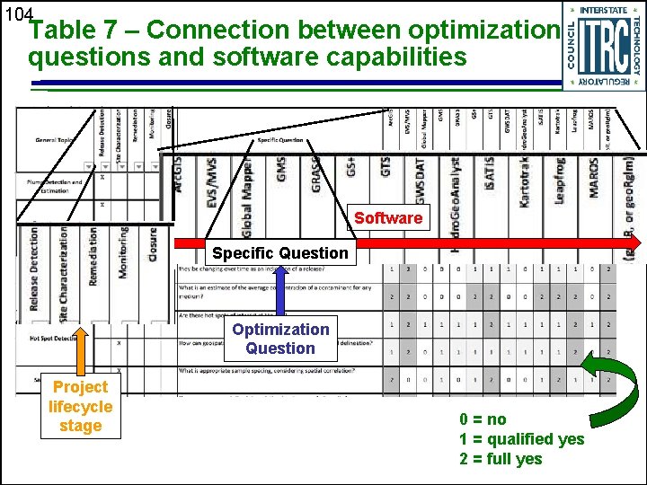
104 Table 7 – Connection between optimization questions and software capabilities Software Specific Question Optimization Question Project lifecycle stage 0 = no 1 = qualified yes 2 = full yes

105 Using Analysis Results for Optimization

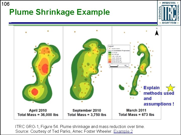
106 Plume Shrinkage Example Explain methods used and assumptions ! ITRC GRO-1, Figure 54. Plume shrinkage and mass reduction over time. Source: Courtesy of Ted Parks, Amec Foster Wheeler. Example 2

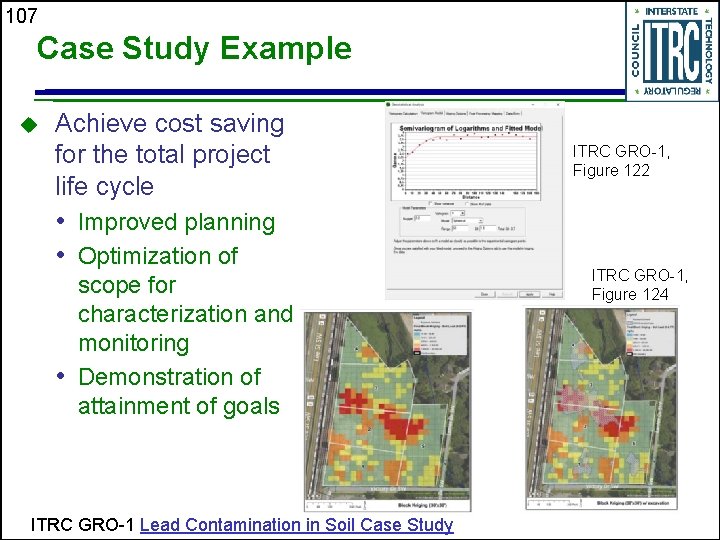
107 Case Study Example Achieve cost saving for the total project life cycle • Improved planning • Optimization of scope for characterization and monitoring • Demonstration of attainment of goals ITRC GRO-1 Lead Contamination in Soil Case Study ITRC GRO-1, Figure 122 ITRC GRO-1, Figure 124

108 Wrap-Up: Geospatial Analyses Geospatial analyses optimize our work, facilitate interpretation/communication The guidance and training mean to encourage proper use of geospatial analyses Geospatial analyses help optimize actions throughout the project life cycle The data must exhibit spatial correlation in order to use geospatial methods All geospatial methods can be used to make maps, but only the more complex or advanced methods can provide estimates of uncertainty

109 Data Interpolation is Method Dependent! ITRC GRO-1, Figure 15, Source: (Kresic and Mikszewski 2012)

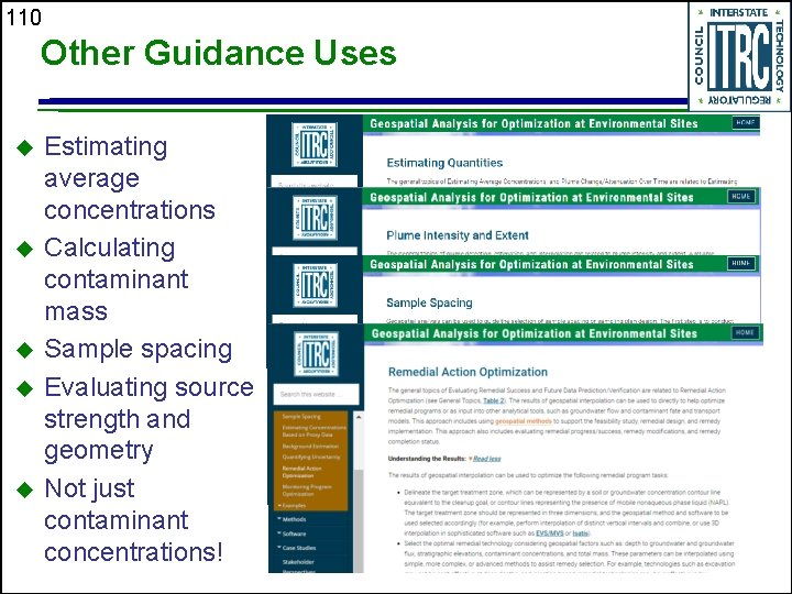
110 Other Guidance Uses Estimating average concentrations Calculating contaminant mass Sample spacing Evaluating source strength and geometry Not just contaminant concentrations!

111 Thank You for Participating 2 nd question and answer break Links to additional resources Poll Questions • http: //www. clu-in. org/conf/itrc/gro/resource. cfm Feedback form – please complete • http: //www. clu-in. org/conf/itrc/gro/feedback. cfm Need confirmation of your participation today? Fill out the feedback form and check box for confirmation email and certificate.