The Use of Semidefinite Programming in Approximation Algorithms

The Use of Semidefinite Programming in Approximation Algorithms Uriel Feige The Weizmann Institute

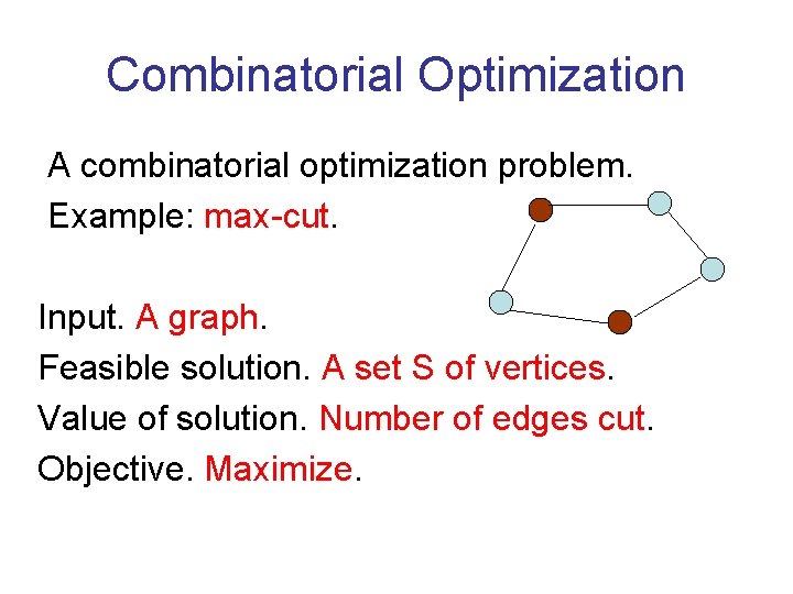
Combinatorial Optimization A combinatorial optimization problem. Example: max-cut. Input. A graph. Feasible solution. A set S of vertices. Value of solution. Number of edges cut. Objective. Maximize.

Coping with NP-hardness Finding the optimal solution is NP-hard. Practical implication: no polynomial time algorithm always finds optimum solution. Approximation algorithms: polynomial time, guaranteed to find “near optimal” solutions for every input. Heuristics: useful algorithmic ideas that often work, but fail on some inputs.

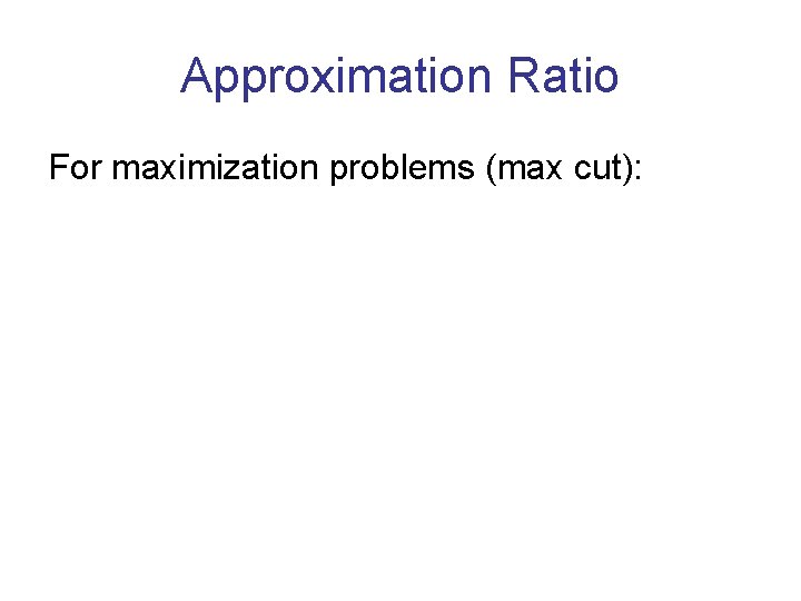
Approximation Ratio For maximization problems (max cut):

A diverse picture Many approximation algorithms designed, for many combinatorial optimization problems, using a variety of algorithmic techniques. A large variation between approximation ratios of different problems. (PTAS, constant, super-constant, logarithmic, polynomial, trivial. )

Hardness of Approximation How can we tell if there is room for further improvement in the approximation ratio? NP-hardness of approximation: improving over an approximation ratio implies P=NP. “Gap preserving” reductions. The PCP theorem. Hardness of approximation under other assumptions.

State of the art Tight thresholds: k-center, max-coverage, max 3 SAT. Reasonable bounds: max 2 SAT, max-cut, min vertex cover. Poor bounds: min bisection. Almost no progress: max bipartite clique. Inapproximable: max clique, longest directed path.

Semidefinite Programming A generalization of linear programming. Most effective for maximization problems involving constraints over pairs of variables. Leads to reasonably good approximation ratios, though in most cases they are not known to be best possible.

In this talk The use of SDP for max-cut. Main result – Goemans and Williamson. But will survey much more. The use of SDP for other problems. Impractical to fully cover (and understand) in three hours. Will mention references for additional reading.

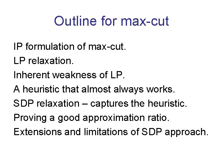
Outline for max-cut IP formulation of max-cut. LP relaxation. Inherent weakness of LP. A heuristic that almost always works. SDP relaxation – captures the heuristic. Proving a good approximation ratio. Extensions and limitations of SDP approach.

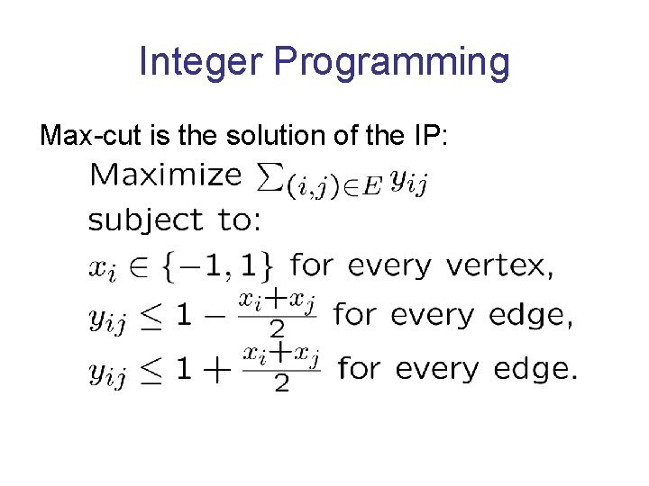
Integer Programming Max-cut is the solution of the IP:

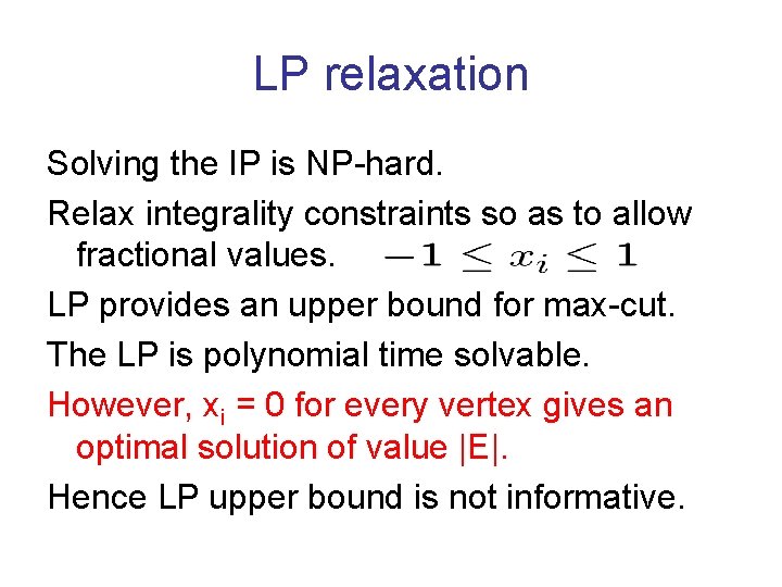
LP relaxation Solving the IP is NP-hard. Relax integrality constraints so as to allow fractional values. LP provides an upper bound for max-cut. The LP is polynomial time solvable. However, xi = 0 for every vertex gives an optimal solution of value |E|. Hence LP upper bound is not informative.

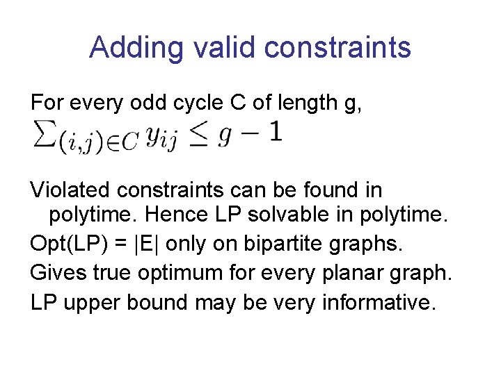
Adding valid constraints For every odd cycle C of length g, Violated constraints can be found in polytime. Hence LP solvable in polytime. Opt(LP) = |E| only on bipartite graphs. Gives true optimum for every planar graph. LP upper bound may be very informative.

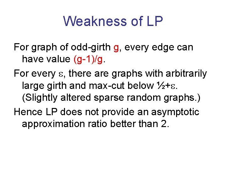
Weakness of LP For graph of odd-girth g, every edge can have value (g-1)/g. For every , there are graphs with arbitrarily large girth and max-cut below ½+. (Slightly altered sparse random graphs. ) Hence LP does not provide an asymptotic approximation ratio better than 2.

Good heuristics For almost all graphs with n vertices, and dn edges, where d is a large enough constant, the value of the LP is almost a factor of 2 away from maxcut. Is there a good heuristic that provides a nearly tight upper bound on most such graphs?

Algebraic Graph Theory A graph can be represented by its adjacency matrix. This is a square symmetric matrix with nonnegative entries. It has only real eigenvalues and eigenvectors. Eigenvalues can be computed in polytime.

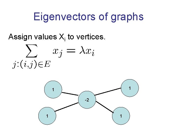
Eigenvectors of graphs Assign values Xi to vertices. 1 1 -2 1 1

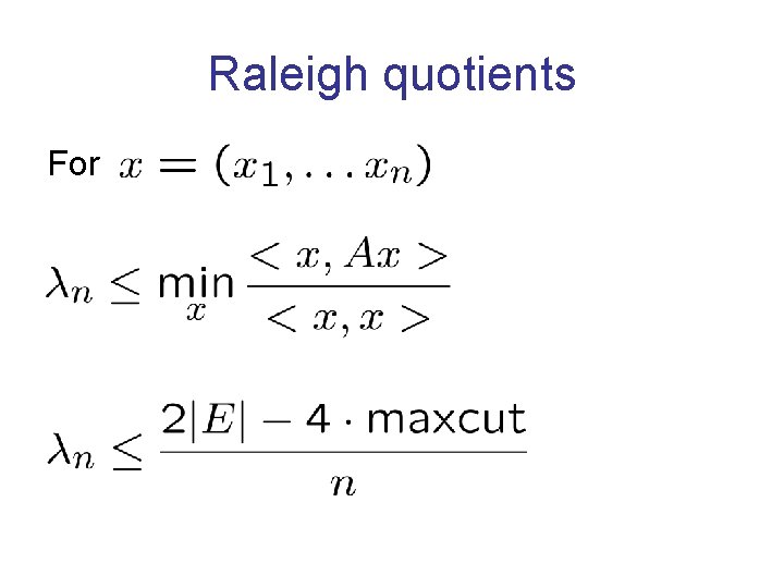
Raleigh quotients For

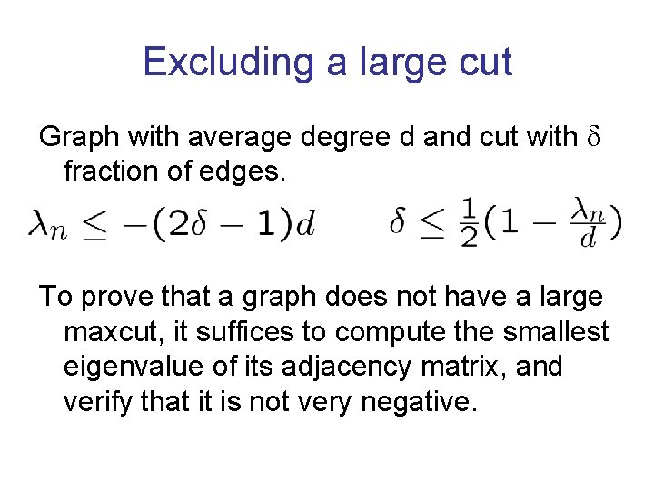
Excluding a large cut Graph with average degree d and cut with fraction of edges. To prove that a graph does not have a large maxcut, it suffices to compute the smallest eigenvalue of its adjacency matrix, and verify that it is not very negative.

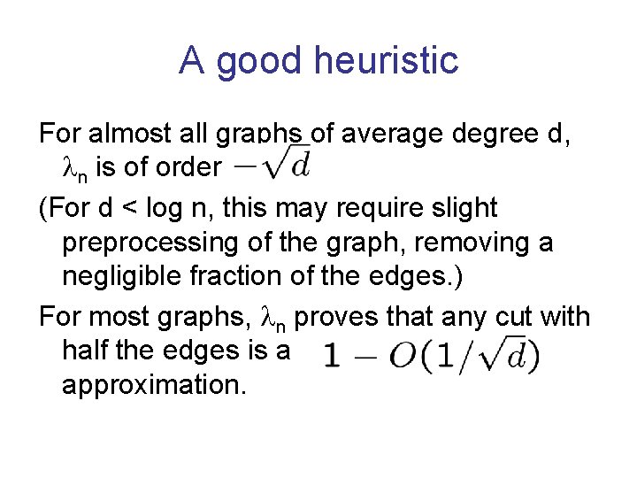
A good heuristic For almost all graphs of average degree d, n is of order (For d < log n, this may require slight preprocessing of the graph, removing a negligible fraction of the edges. ) For most graphs, n proves that any cut with half the edges is a approximation.

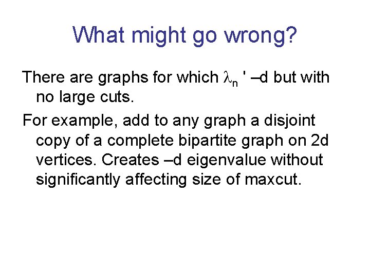
What might go wrong? There are graphs for which n ' –d but with no large cuts. For example, add to any graph a disjoint copy of a complete bipartite graph on 2 d vertices. Creates –d eigenvalue without significantly affecting size of maxcut.

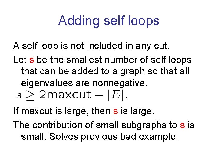
Adding self loops A self loop is not included in any cut. Let s be the smallest number of self loops that can be added to a graph so that all eigenvalues are nonnegative. If maxcut is large, then s is large. The contribution of small subgraphs to s is small. Solves previous bad example.

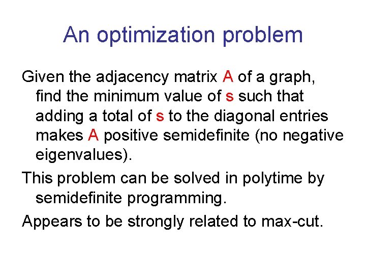
An optimization problem Given the adjacency matrix A of a graph, find the minimum value of s such that adding a total of s to the diagonal entries makes A positive semidefinite (no negative eigenvalues). This problem can be solved in polytime by semidefinite programming. Appears to be strongly related to max-cut.

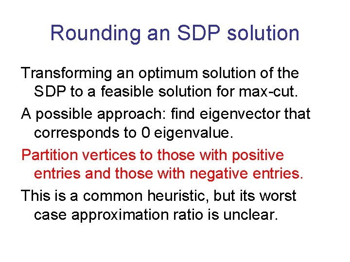
Rounding an SDP solution Transforming an optimum solution of the SDP to a feasible solution for max-cut. A possible approach: find eigenvector that corresponds to 0 eigenvalue. Partition vertices to those with positive entries and those with negative entries. This is a common heuristic, but its worst case approximation ratio is unclear.

References Boppana [FOCS 87]. For most graphs with a cut containing significantly more than half the edges, the SDP heuristic finds the exact max cut. Feige and Kilian [JCSS 2001]. Extensions to more graphs and to other problems.

Goemans and Williamson [JACM 95] Showed how to get from the SDP provably good approximation ratios for max-cut. A minimization SDP has a dual maximization SDP of the same value. The dual SDP in our case (after a linear transformation on the objective function) can also be viewed as a relaxation for an integer quadratic program for maxcut.

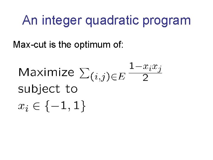
An integer quadratic program Max-cut is the optimum of:

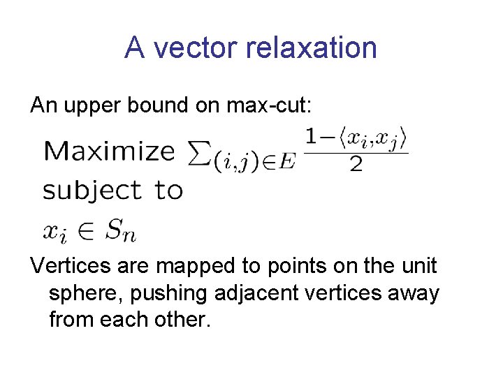
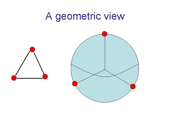
A vector relaxation An upper bound on max-cut: Vertices are mapped to points on the unit sphere, pushing adjacent vertices away from each other.

A geometric view .

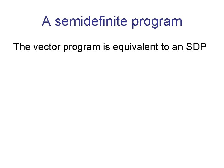
A semidefinite program The vector program is equivalent to an SDP

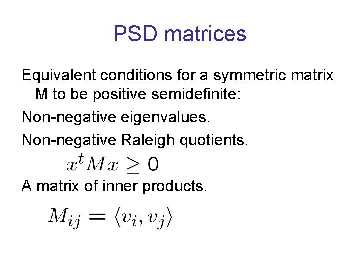
PSD matrices Equivalent conditions for a symmetric matrix M to be positive semidefinite: Non-negative eigenvalues. Non-negative Raleigh quotients. A matrix of inner products.

Rounding an SDP solution A feasible solution to the SDP associates with every vertex a unit vector in , or a point on the unit sphere. A feasible solution to max cut associates with every vertex a unit vector in , or a value. Need a rounding process that does not lose much in value of SDP.

Using geometry of SDP Optimal solution of SDP tends to send adjacent vertices to antipodal points, so as to maximize (1–xixj)/2. Needs a rounding technique that keeps most far away pairs separated, and hence keeps together close pairs. Geometrically, the best choice is a halfsphere. (Isoperimetric inequalities. )

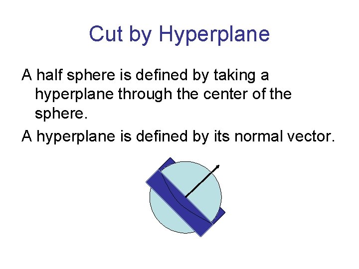
Cut by Hyperplane A half sphere is defined by taking a hyperplane through the center of the sphere. A hyperplane is defined by its normal vector.

Random hyperplane There are infinitely many hyperplanes. Which is the best one for a particular solution to the SDP? Surprise: it does not really matter. Just choose one at random. This partitions sphere in two. Two vertices are on same side of cut if their corresponding points are on the same side of the hyperplane.

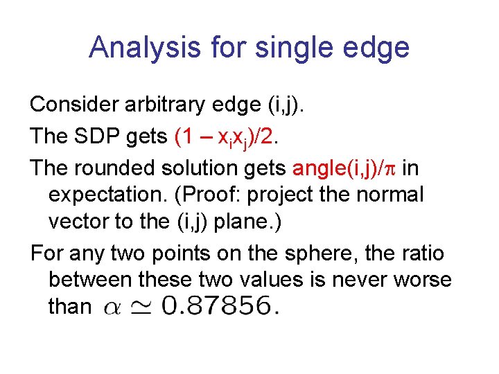
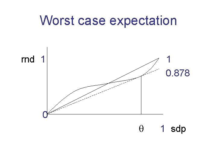
Analysis for single edge Consider arbitrary edge (i, j). The SDP gets (1 – xixj)/2. The rounded solution gets angle(i, j)/ in expectation. (Proof: project the normal vector to the (i, j) plane. ) For any two points on the sphere, the ratio between these two values is never worse than

Worst case expectation rnd 1 1 0. 878 0 1 sdp

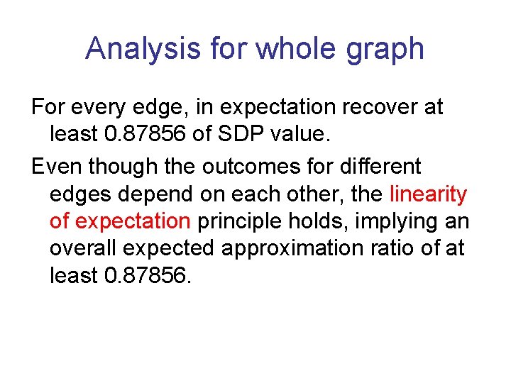
Analysis for whole graph For every edge, in expectation recover at least 0. 87856 of SDP value. Even though the outcomes for different edges depend on each other, the linearity of expectation principle holds, implying an overall expected approximation ratio of at least 0. 87856.

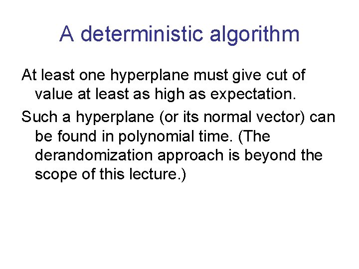
A deterministic algorithm At least one hyperplane must give cut of value at least as high as expectation. Such a hyperplane (or its normal vector) can be found in polynomial time. (The derandomization approach is beyond the scope of this lecture. )

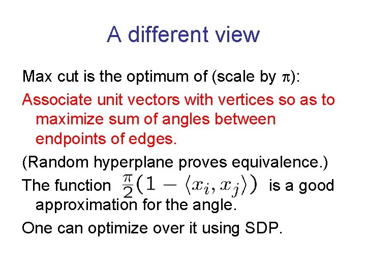
A different view Max cut is the optimum of (scale by ): Associate unit vectors with vertices so as to maximize sum of angles between endpoints of edges. (Random hyperplane proves equivalence. ) The function is a good approximation for the angle. One can optimize over it using SDP.

Summary Naïve approaches (including LP) approximate max cut within a ratio of ½. On almost all graphs, the most negative eigenvalue provides upper bounds that are close to true max-cut. Eigenvalues are sensitive to small changes, and can be fooled in worst case graphs. SDP generalizes eigenvalue techniques.

Summary continued SDP dual gives a maximization problem in which vertices are mapped to points on unit sphere. Random hyperplane through the origin produces a true cut of expected value not far from value of SDP. One can efficiently find a hyperplane giving a cut of value at least the expectation.

Some questions Can we do better than random hyperplane? Can a different SDP produce better approximations for max cut? What other problems have good approximations based on semidefinite programs?

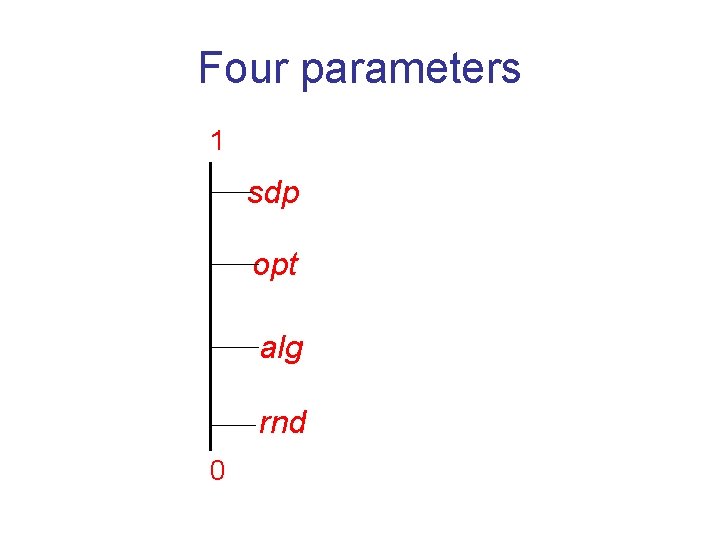
Four parameters 1 sdp opt alg rnd 0

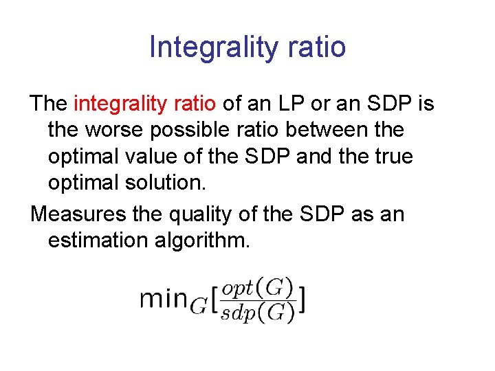
Integrality ratio The integrality ratio of an LP or an SDP is the worse possible ratio between the optimal value of the SDP and the true optimal solution. Measures the quality of the SDP as an estimation algorithm.

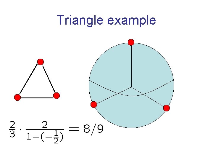
Triangle example .

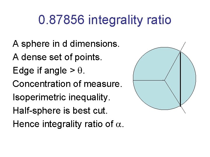
0. 87856 integrality ratio A sphere in d dimensions. A dense set of points. Edge if angle > . Concentration of measure. Isoperimetric inequality. Half-sphere is best cut. Hence integrality ratio of . .

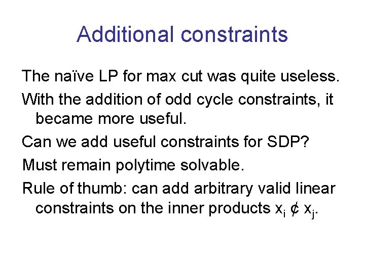
Additional constraints The naïve LP for max cut was quite useless. With the addition of odd cycle constraints, it became more useful. Can we add useful constraints for SDP? Must remain polytime solvable. Rule of thumb: can add arbitrary valid linear constraints on the inner products xi ¢ xj.

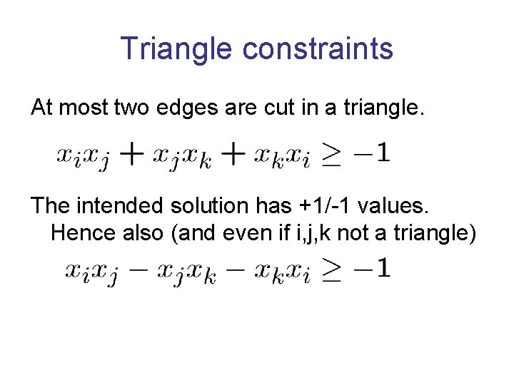
Triangle constraints At most two edges are cut in a triangle. The intended solution has +1/-1 values. Hence also (and even if i, j, k not a triangle)

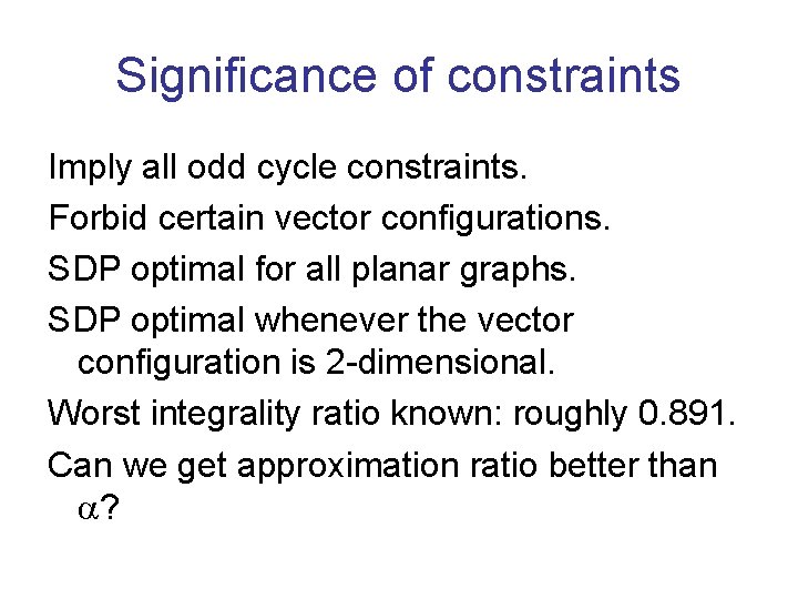
Significance of constraints Imply all odd cycle constraints. Forbid certain vector configurations. SDP optimal for all planar graphs. SDP optimal whenever the vector configuration is 2 -dimensional. Worst integrality ratio known: roughly 0. 891. Can we get approximation ratio better than ?

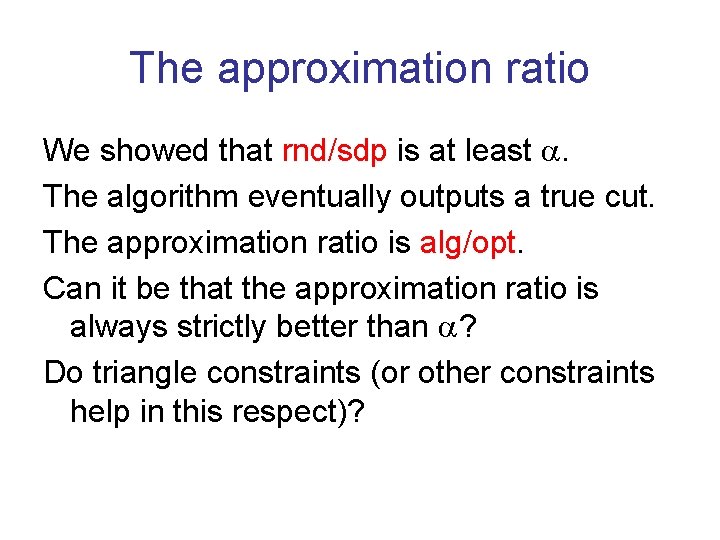
The approximation ratio We showed that rnd/sdp is at least . The algorithm eventually outputs a true cut. The approximation ratio is alg/opt. Can it be that the approximation ratio is always strictly better than ? Do triangle constraints (or other constraints help in this respect)?

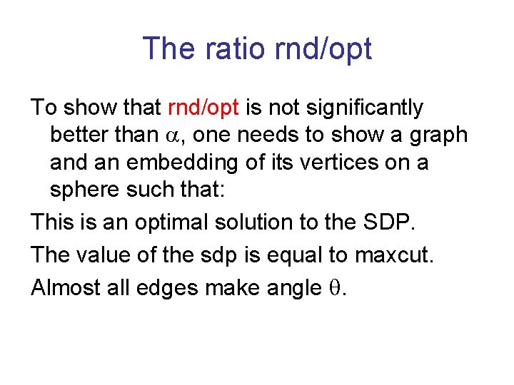
The ratio rnd/opt To show that rnd/opt is not significantly better than , one needs to show a graph and an embedding of its vertices on a sphere such that: This is an optimal solution to the SDP. The value of the sdp is equal to maxcut. Almost all edges make angle .

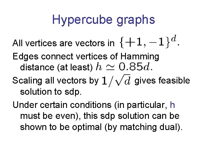
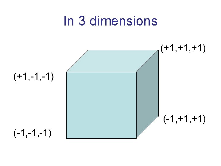
Hypercube graphs All vertices are vectors in Edges connect vertices of Hamming distance (at least) Scaling all vectors by gives feasible solution to sdp. Under certain conditions (in particular, h must be even), this sdp solution can be shown to be optimal (by matching dual).

In 3 dimensions (+1, +1) (+1, -1) (-1, +1) (-1, -1)

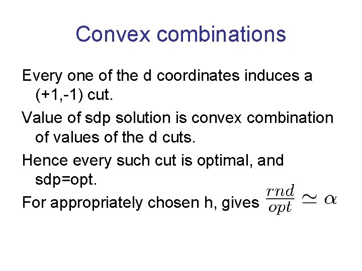
Convex combinations Every one of the d coordinates induces a (+1, -1) cut. Value of sdp solution is convex combination of values of the d cuts. Hence every such cut is optimal, and sdp=opt. For appropriately chosen h, gives

Additional constraints Hypercube embedding is a convex combination of true cuts. True cuts satisfy all “reasonable” constraints. Hypercube embeddings satisfy all reasonable (including triangle) constraints. Negative example applies without change.

Best hyperplane The hyperplane eventually chosen by the algorithm is not random. Hence potentially, alg > rnd. Hypercube graphs can be generalized to show that even best hyperplane does not give approximation ratio better than .

Summary Max-cut can be formulated as SDP. Random hyperplane within of sdp. Integrality ratio opt/sdp might be . Approximation ratio alg/opt might be . It is an open question whether triangle constraints improve integrality ratio beyond . Need different rounding technique.

References Karloff [SICOMP 99] shows that for the hypercube, the natural embedding is an optimal solution to the SDP. Feige and Schechtman [RSA 02] provide an extensive discussion of the integrality ratio and the approximation ratio for max cut.

Special cases Approximation ratio better than : Graphs with very large cuts. Graphs with only small cuts. Very dense graphs. Very sparse graphs.

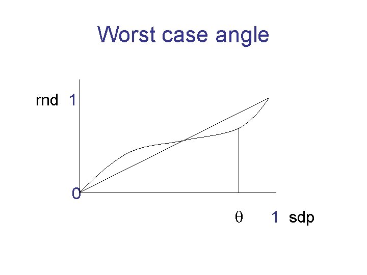
Worst case angle rnd 1 0 1 sdp

Useful principle Favorable solution of SDP: a significant part of the weight of the solution comes from edges whose angle significantly differs from . Then the expected size of a cut given by a random hyperplane is significantly above an fraction of sdp.

Heavy max-cut (> 0. 844) Say opt > 0. 99. Then sdp > 0. 99. Then typical edges contribute > 0. 99 to sdp. This corresponds to an angle > . Random hyperplane expected to recover more than fraction of their value. Approximation ratio > .

Light max-cut (< 0. 844) Say sdp < 0. 7. Then typical edges contribute < 0. 7 to sdp. This corresponds to an angle < . Random hyperplane expected to recover more than fraction of their value. Approximation ratio > .

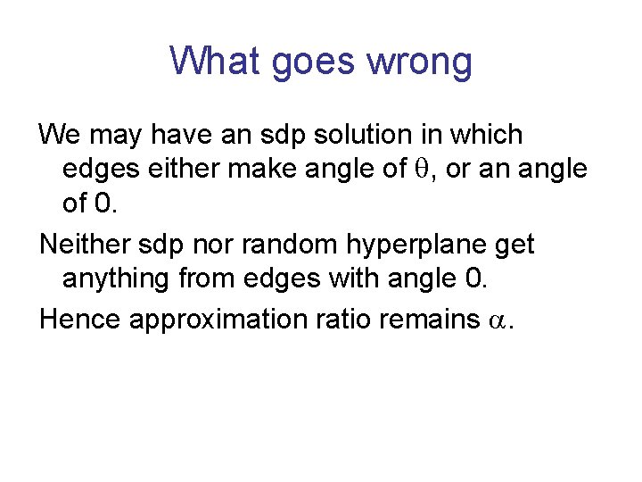
What goes wrong We may have an sdp solution in which edges either make angle of , or an angle of 0. Neither sdp nor random hyperplane get anything from edges with angle 0. Hence approximation ratio remains .

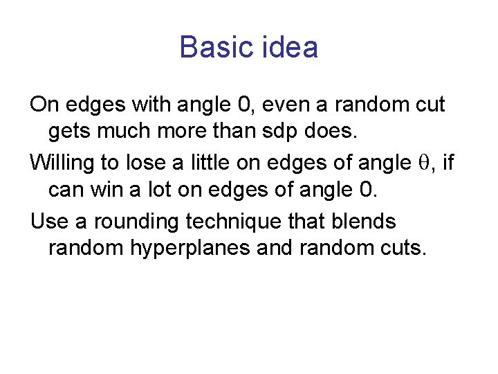
Basic idea On edges with angle 0, even a random cut gets much more than sdp does. Willing to lose a little on edges of angle , if can win a lot on edges of angle 0. Use a rounding technique that blends random hyperplanes and random cuts.

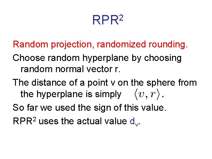
RPR 2 Random projection, randomized rounding. Choose random hyperplane by choosing random normal vector r. The distance of a point v on the sphere from the hyperplane is simply So far we used the sign of this value. RPR 2 uses the actual value dv.

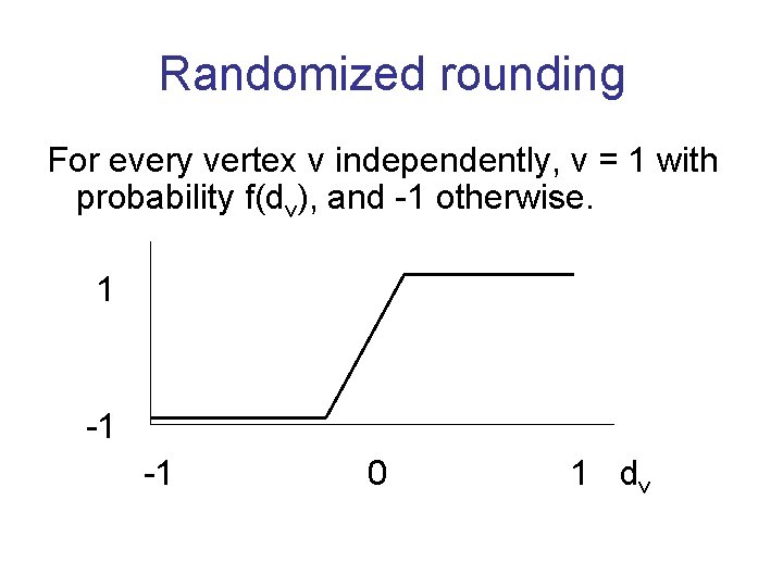
Randomized rounding For every vertex v independently, v = 1 with probability f(dv), and -1 otherwise. 1 -1 -1 0 1 dv

The rounding function f The optimal choice of f depends on the value sdp. For lower sdp, lower slope. Near-optimal choice is piecewise linear. Computer assisted analysis to find best “worst case” approximation ratio.

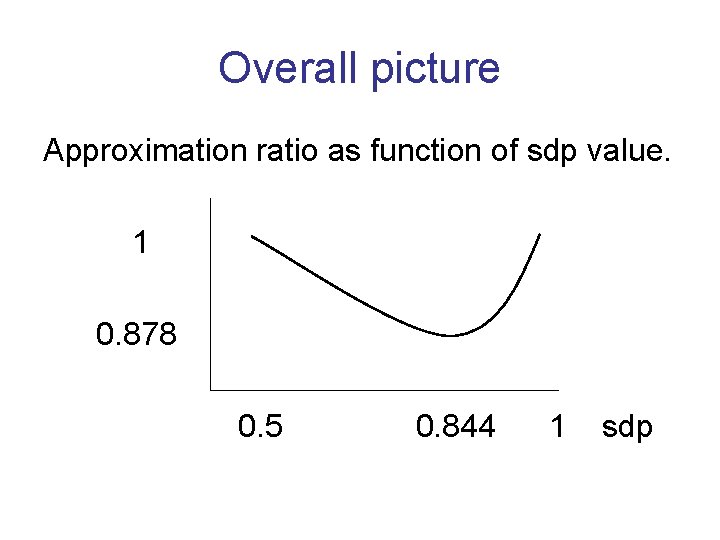
Overall picture Approximation ratio as function of sdp value. 1 0. 878 0. 5 0. 844 1 sdp

References Heavy max-cut was already analysed by Goemans and Williamson. Light max-cut was first analysed by Zwick [STOC 99], using outward rotations. The RPR 2 technique was introduced by Feige and Langberg [ICALP 01].

Biased vertices For the maximum cut, a vertex is biased if significantly more than half its neighbors are on the other side. Intuitively, if we could recognize (most) biased vertices and place them correctly, then we will get a near optimal cut. We can afford to make mistakes with the unbiased vertices.

Dense graphs Number of edges (n 2). Assume for simplicity that all degrees > n/2. Pick at random O(log n) vertices, and guess on which side of the cut they are (try all possibilities). For the correct guess, majority vote will then place correctly almost all biased vertices. With extra work, get a PTAS.

Sparse graphs Graphs with O(n) edges. Assume for simplicity that all degrees < d. Even without SDP can guarantee approximation ratio > ½ + (1/d) (homework). With SDP can get approximation ratio better than + (1/d 4). For degree < 4, approximation ratio > 0. 92.

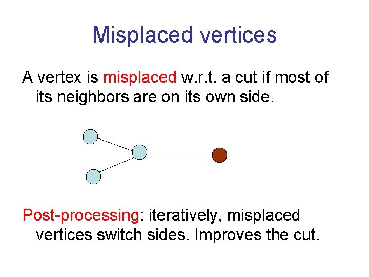
Misplaced vertices A vertex is misplaced w. r. t. a cut if most of its neighbors are on its own side. Post-processing: iteratively, misplaced vertices switch sides. Improves the cut.

Desirable situation For post-processing to improve approximation ratio of an algorithm: A constant fraction of the vertices need to be misplaced by the algorithm. Switching a misplaced vertex needs to contribute (1/n) to the cut. Secondition holds for bounded degree graphs.

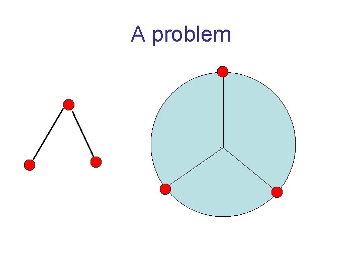
Misplaced vertices for SDP In general, random hyperplane might not produce any misplaced vertices, and postprocessing does not help. However, we are interested only in the following case: - Maximum degree is d. - (most) angles are .

A problem .

Solution Add triangle constraints. They forbid certain vector configurations. Lemma: for every pair of edges (u, v), (u, w), with angles roughly (and M constraints), random hyperplane places u, v, w on same side with constant probability. If d=2, 3, this means that u is misplaced. For d > 3, more work is needed.

References Dense max-cut (and dense instances of other problems) was considered by Arora, Karger and Karpinski [JCSS 99], and by others. Sparse max-cut is analysed in Feige, Karpinski and Langberg [JALG 02].

Summary for max-cut SDP + random hyperplane give ratio . If opt > 0. 844 then ratio improves. If opt < 0. 844 then ratio improves with RPR 2. If |E| = (n 2), PTAS using sampling. If |E| = O(n), improvement using triangle constraints and post-processing. Known hardness of approximation: 16/17.

Related problems We shall survey the use of SDP for approximating some other problems. Some new ideas involved. Some cases where SDP looks like it may work, but it does not seem to work well enough.

Weighted instances In weighted max-cut, edges have nonnegative weights, and one seeks a cut of maximum weight. SDP (with weighted objective function) leads to the same approximation ratio . This is a common phenomenon for approximation algorithms based on LP or SDP.

Min bipartization The complement of max-cut. Remove the smallest number of edges so that the graph becomes bipartite. Not known to be approximable within constant factors. If opt = 2 |E| , SDP for max-cut + random hyperplane might pay |E|. Approximation ratio as bad as 1/. (See homework. )

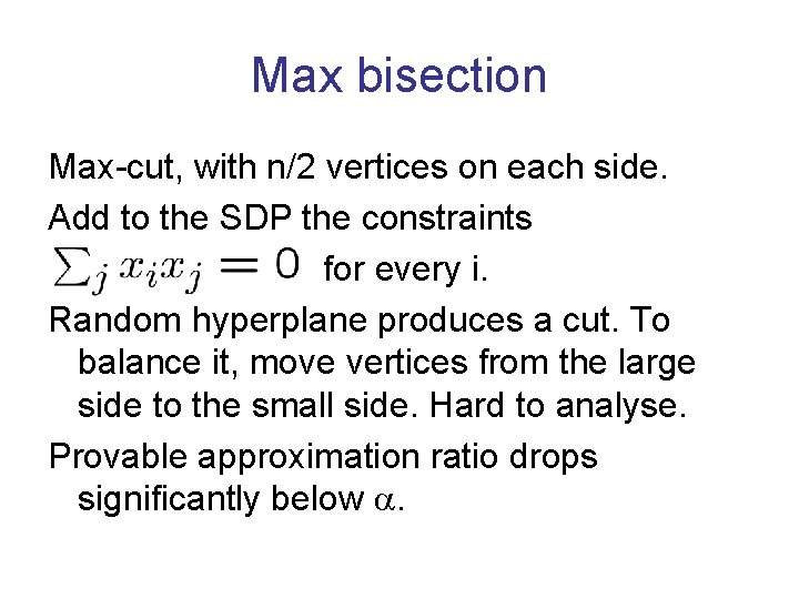
Max bisection Max-cut, with n/2 vertices on each side. Add to the SDP the constraints for every i. Random hyperplane produces a cut. To balance it, move vertices from the large side to the small side. Hard to analyse. Provable approximation ratio drops significantly below .

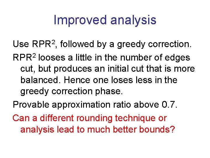
Improved analysis Use RPR 2, followed by a greedy correction. RPR 2 looses a little in the number of edges cut, but produces an initial cut that is more balanced. Hence one loses less in the greedy correction phase. Provable approximation ratio above 0. 7. Can a different rounding technique or analysis lead to much better bounds?

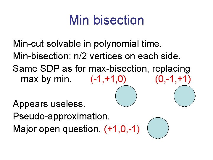
Min bisection Min-cut solvable in polynomial time. Min-bisection: n/2 vertices on each side. Same SDP as for max-bisection, replacing max by min. (-1, +1, 0) (0, -1, +1) Appears useless. Pseudo-approximation. Major open question. (+1, 0, -1)

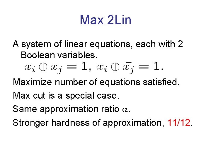
Max 2 Lin A system of linear equations, each with 2 Boolean variables. Maximize number of equations satisfied. Max cut is a special case. Same approximation ratio . Stronger hardness of approximation, 11/12.

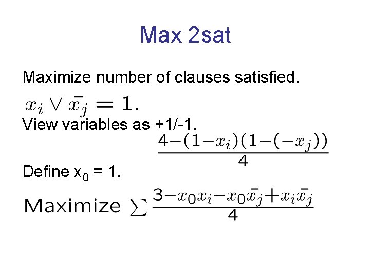
Max 2 sat Maximize number of clauses satisfied. View variables as +1/-1. Define x 0 = 1.

Rounding technique Allow variables to be arbitrary unit vectors. Solve SDP. Take random hyperplane. Give literals on same side of x 0 value 1, and their complements value 0. Approximation ratio , same as max-cut (though analysis more difficult).

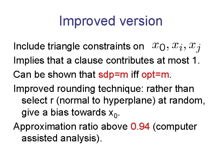
Improved version Include triangle constraints on Implies that a clause contributes at most 1. Can be shown that sdp=m iff opt=m. Improved rounding technique: rather than select r (normal to hyperplane) at random, give a bias towards x 0. Approximation ratio above 0. 94 (computer assisted analysis).

References Max 2 sat was already considered by Goemans and Williamson. Triangle constraints were added analysed (using rotations) by Feige and Goemans [ISTCS 95]. Best current bounds, Lewin, Livnat and Zwick [IPCO 02].

Some other problems Color 3 -color graphs with (m/n)1/3 colors. Gives a bound on the size of MIS (the Lovasz theta function). Does not appear to give an approximation ratio better than 2 for vertex cover. Tight approximation ratio 7/8 for max 3 sat.

References 3 -coloring: Karger, Motwani and Sudan [JACM 98]. Independent set: Alon and Kahale [Math. Programming 98]. Vertex cover: Charikar [SODA 02]. Max 3 SAT: Karloff and Zwick [FOCS 97]. Many more works on SDP. Hardness results: Hastad [JACM 01].

Summary SDP produces the best known approximation ratios for many maximization problems involving 2 variables per constraint. Computer assisted design and analysis of approximation ratio is quite common. Often, there are no known matching hardness of approximation results.