Steiner Forest V V Vazirani Approximation Algorithms Chapters

Steiner Forest V. V. Vazirani. Approximation Algorithms Chapters 3 & 22 Jennifer Campbell 2010/11/07

Overview Steiner Tree (chp 3) Steiner Trees Metric Steiner Trees Steiner Forest (chp 22) Definition LP-relaxation and dual Primal-dual with synchronization Example Analysis

Steiner Tree Defined by Gauss in a letter he wrote to Schumacher A problem in combinatorial optimization Similar to Min. Spanning Tree. Difference is the use of intermediate vertices and edges to reduce the length of the spanning tree

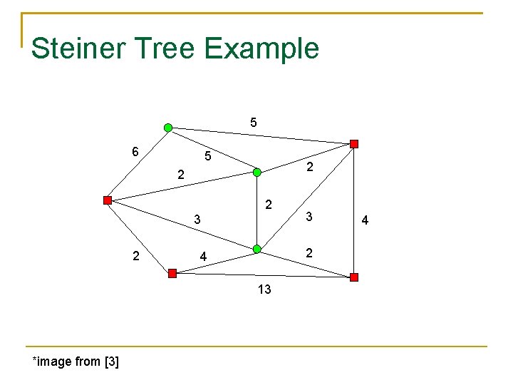
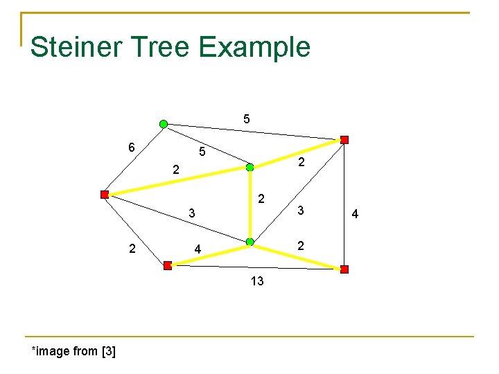
Steiner Tree Definition Given an undirected graph G=(V, E) with nonegative edge costs and whose vertices are partitioned into two sets, required and Steiner, find a minimum cost tree in G that contains all the required vertices and any subset of the Steiner vertices.

Steiner Tree Example 5 6 5 2 2 2 3 2 2 4 13 *image from [3] 3 4

Steiner Tree Example 5 6 5 2 2 2 3 2 2 4 13 *image from [3] 3 4

Steiner Tree - Applications VLSI design – length of interconnection of terminals computational biology – construction phylogney trees network routing wireless communications

Overview Steiner Tree (chp 3) Steiner Trees Metric Steiner Trees Steiner Forest (chp 22) Definition LP-relaxation and dual Primal-dual with synchronization Example Analysis

Metric Steiner Tree W. L. G. Steiner tree can be turned into a Metric Steiner Tree: The edge costs satisfy the triangle inequality. i. e. , G is a complete undirected graph, and for any three vertices, u, v and w, cost(u, v) ≤ cost(u, w) + cost(v, w)

Metric Steiner Tree (reduction ) Transform, in poly time, an instance I of Steiner tree problem, graph G=(V, E), to an instance I' of a Metric Steiner Tree. The metric closure, G', of G is: Let G' be the complete undirected graph on V. Define the cost of edge (u, v) in G' to the be cost of the shortest u-v path in G. The partition of Steiner and required vertices is the same in I' as in I. Therefore, For any edge (u, v) in E, the cost in G' not more than in G. So cost(OPT) of I' Is not more than cost(OPT) in I

Metric Steiner Tree (reduction ) So, given a Steiner tree T' in I': The cost of edge(u, v) in G' corresponds to the cost of a path in G. Replace each edge of T' by the corresponding path in G. All required vertices are connected, but could contain cycles. Remove edges to options a tree T. Any approximation factor for a Metric Steiner Trees carries over to Steiner trees.

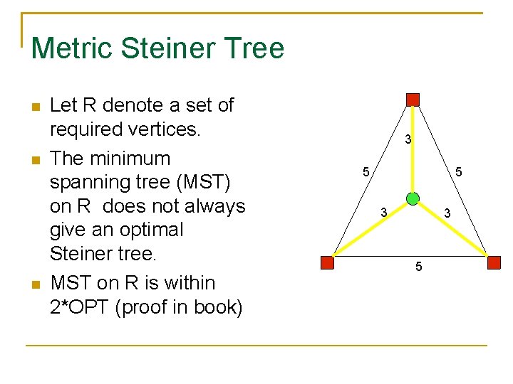
Metric Steiner Tree Let R denote a set of required vertices. The minimum spanning tree (MST) on R does not always give an optimal Steiner tree. MST on R is within 2*OPT (proof in book) 3 5 5 3 3 5

Overview Steiner Tree (chp 3) Steiner Trees Metric Steiner Trees Steiner Forest (chp 22) Definition LP-relaxation and dual Primal-dual with synchronization Example Analysis

Steiner Forest Given an undirected graph G = (V, E), a cost function on edges c: E → Q+, and a collection on disjoint subsets of V, S 1, . . . Sk, find a minimum cost subgraph in which each pair of vertices belonging to the same set Si is connected.

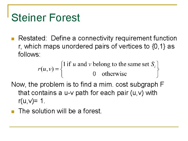
Steiner Forest Restated: Define a connectivity requirement function r, which maps unordered pairs of vertices to {0, 1} as follows: Now, the problem is to find a mim. cost subgraph F that contains a u-v path for each pair (u, v) with r(u, v)= 1. The solution will be a forest.

Steiner Forest Relationship to Steiner Tree: A Steiner Forest with k=1 Since Steiner tree is NP-Hard, Steiner Forest is NP-Hard

Overview Steiner Tree (chp 3) Steiner Trees Metric Steiner Trees Steiner Forest (chp 22) Definition LP-relaxation and dual Primal-dual with synchronization Example Analysis

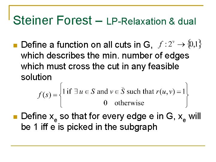
Steiner Forest – LP-Relaxation & dual Define a function on all cuts in G, which describes the min. number of edges which must cross the cut in any feasible solution Define xe so that for every edge e in G, xe will be 1 iff e is picked in the subgraph

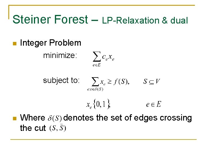
Steiner Forest – LP-Relaxation & dual Integer Problem minimize: subject to: Where the cut denotes the set of edges crossing

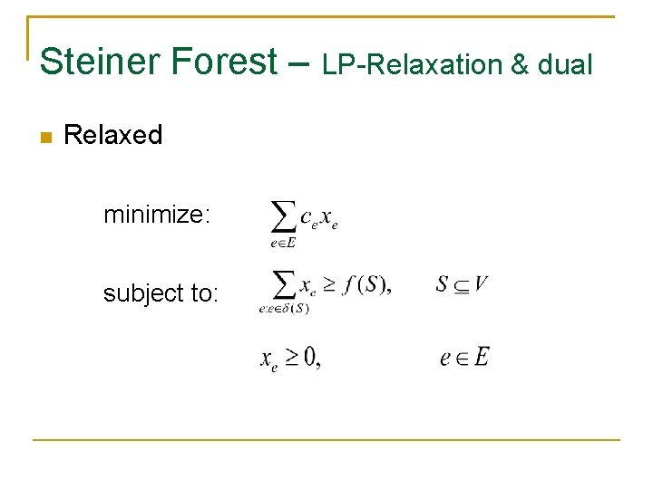
Steiner Forest – LP-Relaxation & dual Relaxed minimize: subject to:

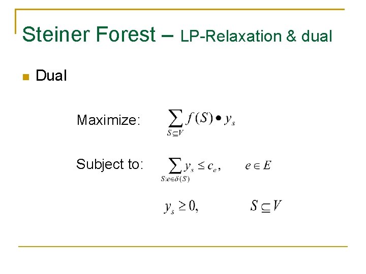
Steiner Forest – LP-Relaxation & dual Dual Maximize: Subject to:

Overview Steiner Tree (chp 3) Steiner Trees Metric Steiner Trees Steiner Forest (chp 22) Definition LP-relaxation and dual Primal-dual with synchronization Example Analysis

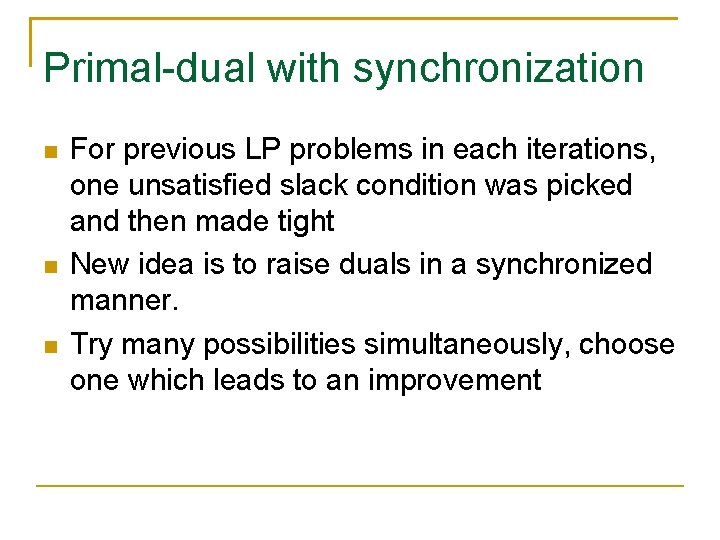
Primal-dual with synchronization For previous LP problems in each iterations, one unsatisfied slack condition was picked and then made tight New idea is to raise duals in a synchronized manner. Try many possibilities simultaneously, choose one which leads to an improvement

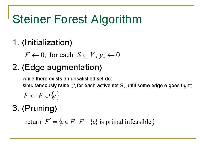
Steiner Forest Algorithm 1. (Initialization) 2. (Edge augmentation) while there exists an unsatisfied set do: simultaneously raise for each active set S, until some edge e goes tight; 3. (Pruning)

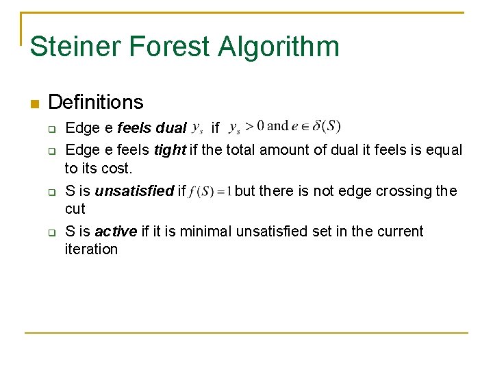
Steiner Forest Algorithm Definitions Edge e feels dual if Edge e feels tight if the total amount of dual it feels is equal to its cost. S is unsatisfied if but there is not edge crossing the cut S is active if it is minimal unsatisfied set in the current iteration

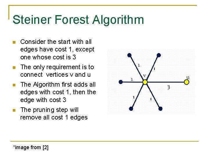
Steiner Forest Algorithm Consider the start with all edges have cost 1, except one whose cost is 3 The only requirement is to connect vertices v and u The Algorithm first adds all edges with cost 1, then the edge with cost 3 The pruning step will remove all cost 1 edges *image from [2]

Overview Steiner Tree (chp 3) Steiner Trees Metric Steiner Trees Steiner Forest (chp 22) Definition LP-relaxation and dual Primal-dual with synchronization Example Analysis

Example Requirements: *image from [2]

Example Optimal solution: 45 *image from [2]

Example: First Iteration *image from [2]

Example: Second Iteration *image from [2]

Example: Third Iteration *image from [2]

Example: Fourth Iteration *image from [2]

Example: Fifth Iteration *image from [2]

Example: Pruning Step Solution: Final cost 54 vs OPT cost 45 *image from [2]

Overview Steiner Tree (chp 3) Steiner Trees Metric Steiner Trees Steiner Forest (chp 22) Definition LP-relaxation and dual Primal-dual with synchronization Example Analysis

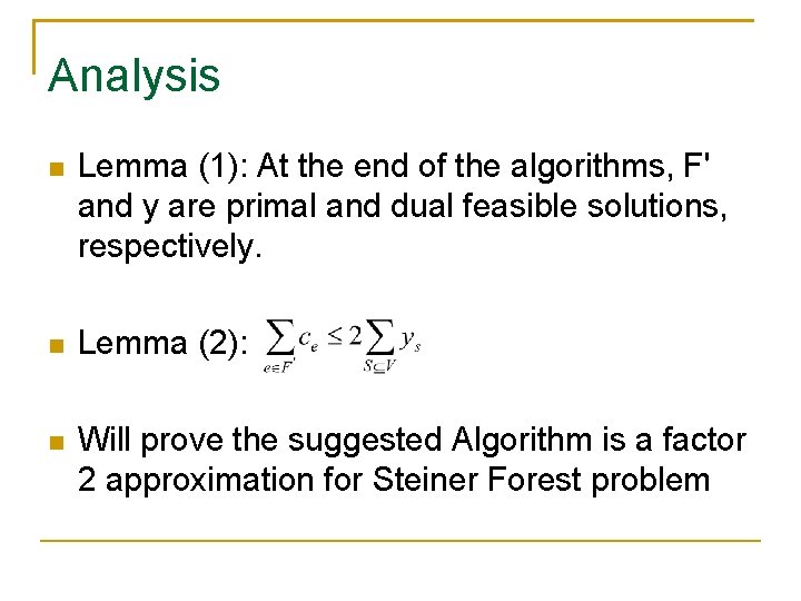
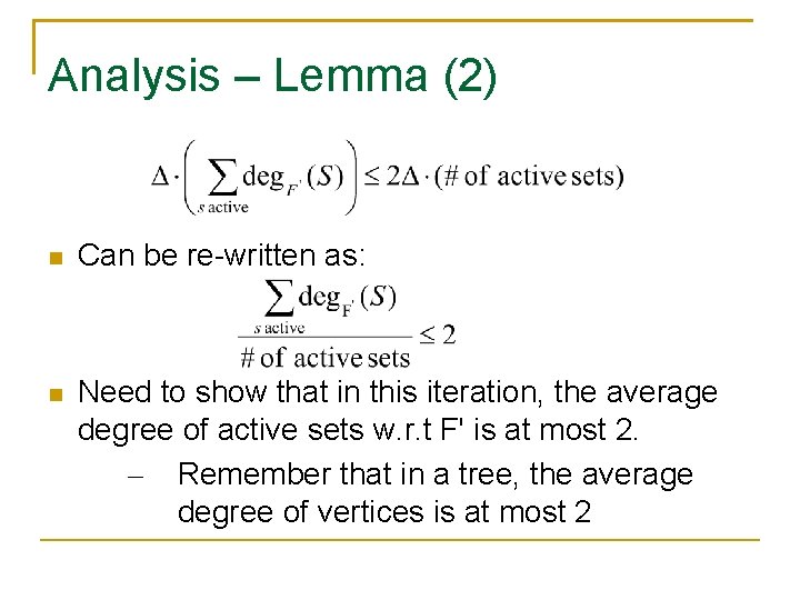
Analysis Lemma (1): At the end of the algorithms, F' and y are primal and dual feasible solutions, respectively. Lemma (2): Will prove the suggested Algorithm is a factor 2 approximation for Steiner Forest problem

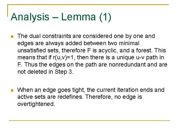
Analysis – Lemma (1) The dual constraints are considered one by one and edges are always added between two minimal unsatisfied sets, therefore F is acyclic, and a forest. This means that if r(u, v)=1, then there is a unique u-v path in F. Thus the edges on the path are nonredundant and are not deleted in Step 3. When an edge goes tight, the current iteration ends and active sets are redefines. Therefore, no edge is overtightened.

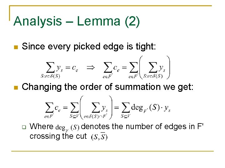
Analysis – Lemma (2) Since every picked edge is tight: Changing the order of summation we get: Where denotes the number of edges in F' crossing the cut

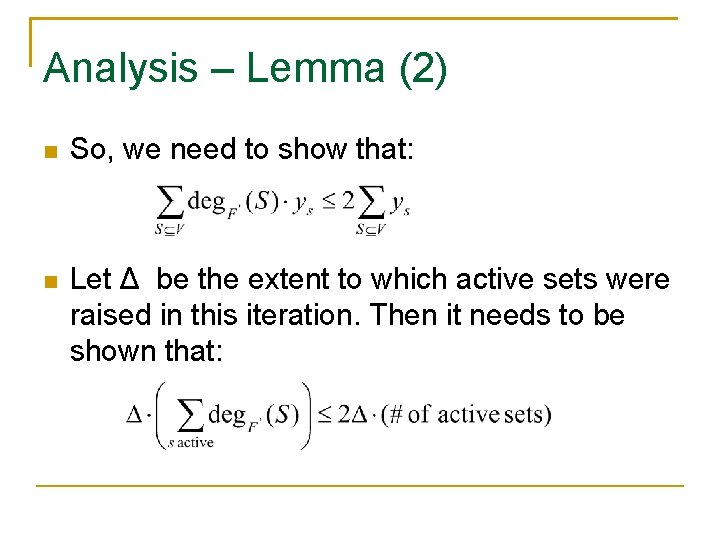
Analysis – Lemma (2) So, we need to show that: Let Δ be the extent to which active sets were raised in this iteration. Then it needs to be shown that:

Analysis – Lemma (2) Can be re-written as: Need to show that in this iteration, the average degree of active sets w. r. t F' is at most 2. – Remember that in a tree, the average degree of vertices is at most 2

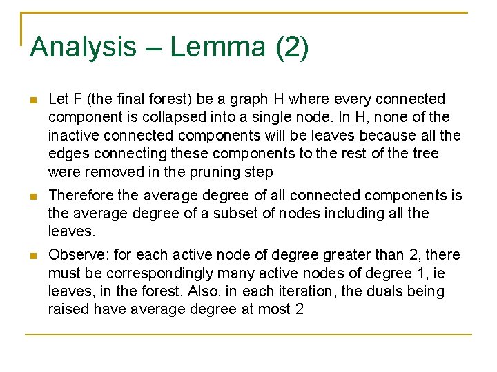
Analysis – Lemma (2) Let F (the final forest) be a graph H where every connected component is collapsed into a single node. In H, none of the inactive connected components will be leaves because all the edges connecting these components to the rest of the tree were removed in the pruning step Therefore the average degree of all connected components is the average degree of a subset of nodes including all the leaves. Observe: for each active node of degree greater than 2, there must be correspondingly many active nodes of degree 1, ie leaves, in the forest. Also, in each iteration, the duals being raised have average degree at most 2

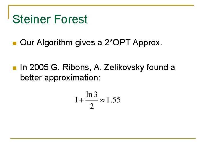
Steiner Forest Our Algorithm gives a 2*OPT Approx. In 2005 G. Ribons, A. Zelikovsky found a better approximation:

References [1] V. V. Vazirani. Approximation Algorithm. Springer, 2003 [2] corelab. ntua. gr. Educational Course. 9 Oct. 2010 <http: //www. corelab. ntua. gr/courses/approx-alg/material/Steiner. Forest. Problem. pdf>. [3] Cheng-Chung Li. 2004. Theoretical Computer Science, The Full Steiner Tree Problem. 28 Jun. 2004. [4] Shuchi Chawla. CS 880: Approximation Algorithms, Primal-Dual Method: Steiner Forest and Facility Location. 8 Mar 2007.