Linear approximation and differentials Section 2 9 Alex

Linear approximation and differentials (Section 2. 9) Alex Karassev

Linear approximation

Problem of computation l l l How do calculators and computers know that √ 5 ≈ 2. 236 or sin 10 o ≈ 0. 173648 ? They use various methods of approximation, one of which is Taylor polynomial approximation A simplest case of Taylor polynomial approximation is linear approximation or linearization

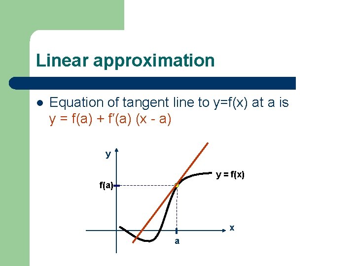
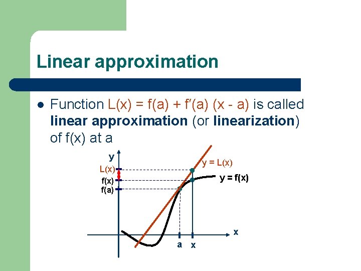
Linear approximation l Equation of tangent line to y=f(x) at a is y = f(a) + f′(a) (x - a) y y = f(x) f(a) x a

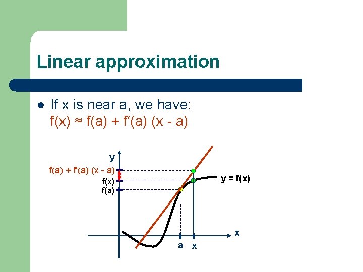
Linear approximation l If x is near a, we have: f(x) ≈ f(a) + f′(a) (x - a) y = f(x) f(a) x a x

Linear approximation l Function L(x) = f(a) + f′(a) (x - a) is called linear approximation (or linearization) of f(x) at a y L(x) y = f(x) f(a) x a x

Example l l Find linearization of f(x) = √x at a Use it to find approximate value of √ 5

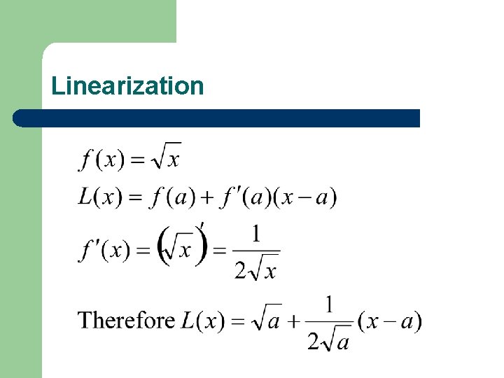
Linearization

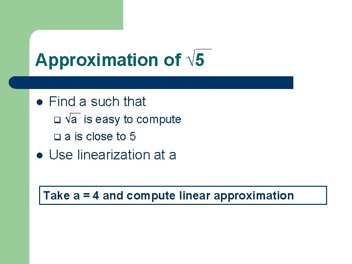
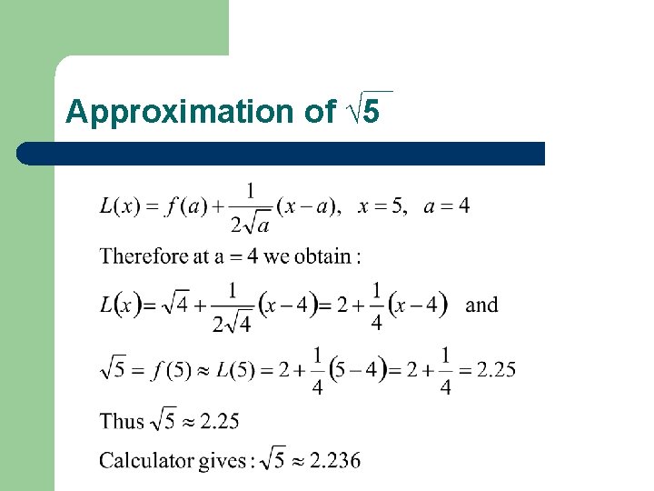
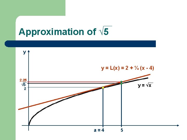
Approximation of √ 5 l Find a such that √a is easy to compute q a is close to 5 q l Use linearization at a Take a = 4 and compute linear approximation

Approximation of √ 5

Approximation of √ 5 y y = L(x) = 2 + ¼ (x - 4) 2. 25 √ 5 y = √x 2 a=4 5

Example l Find approximate value of sin 10 o

Example l l We measure x in radians o So, 10 = 10 (π/180) = π/18 radians Consider f(x) = sin x Find a such that sin(a) is easy to compute q a is near π/18 q Take a = 0 and compute linear approximation

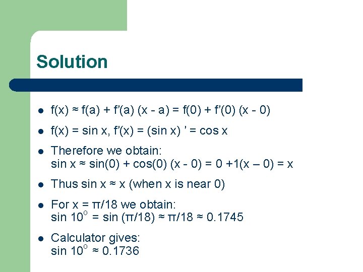
Solution l f(x) ≈ f(a) + f′(a) (x - a) = f(0) + f′(0) (x - 0) l f(x) = sin x, f′(x) = (sin x) ′ = cos x l Therefore we obtain: sin x ≈ sin(0) + cos(0) (x - 0) = 0 +1(x – 0) = x l Thus sin x ≈ x (when x is near 0) l For x = π/18 we obtain: sin 10 o = sin (π/18) ≈ π/18 ≈ 0. 1745 l Calculator gives: sin 10 o ≈ 0. 1736

Differentials

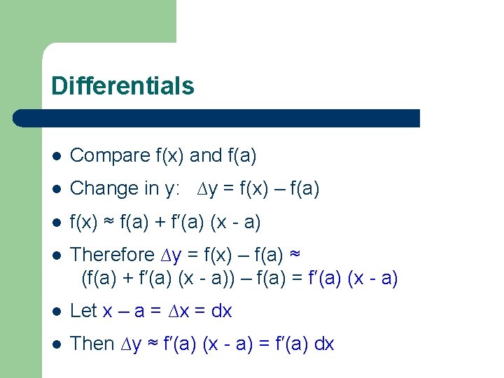
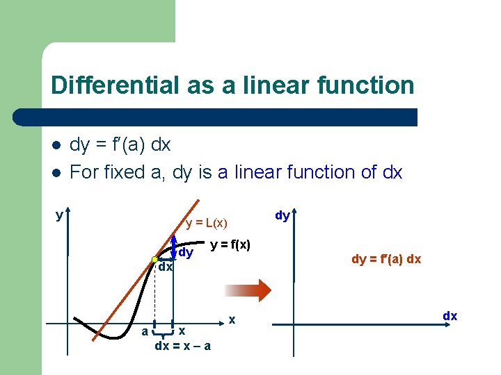
Differentials l Compare f(x) and f(a) l Change in y: ∆y = f(x) – f(a) l f(x) ≈ f(a) + f′(a) (x - a) l Therefore ∆y = f(x) – f(a) ≈ (f(a) + f′(a) (x - a)) – f(a) = f′(a) (x - a) l Let x – a = ∆x = dx l Then ∆y ≈ f′(a) (x - a) = f′(a) dx

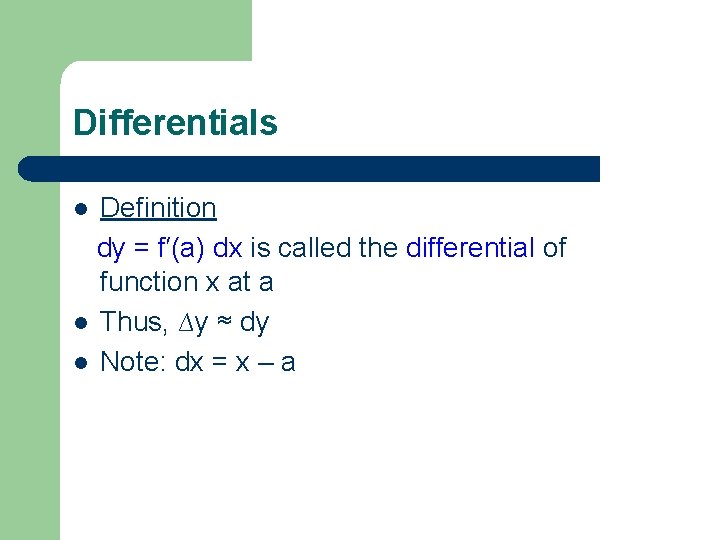
Differentials Definition dy = f′(a) dx is called the differential of function x at a l Thus, ∆y ≈ dy l Note: dx = x – a l

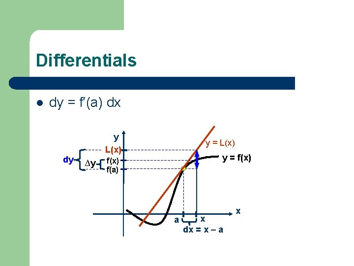
Differentials l dy = f′(a) dx dy y L(x) ∆y y = L(x) y = f(x) f(a) a x dx = x – a x

Differential as a linear function l l dy = f′(a) dx For fixed a, dy is a linear function of dx y dy y = L(x) dy y = f(x) dy = f′(a) dx dx a x dx = x – a x dx

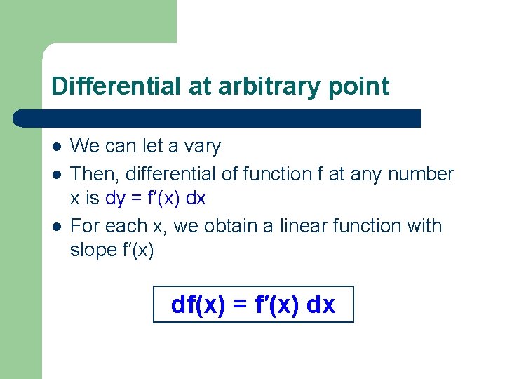
Differential at arbitrary point l l l We can let a vary Then, differential of function f at any number x is dy = f′(x) dx For each x, we obtain a linear function with slope f′(x) df(x) = f′(x) dx

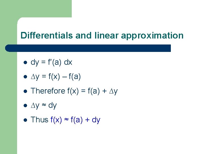
Differentials and linear approximation l dy = f′(a) dx l ∆y = f(x) – f(a) l Therefore f(x) = f(a) + ∆y l ∆y ≈ dy l Thus f(x) ≈ f(a) + dy

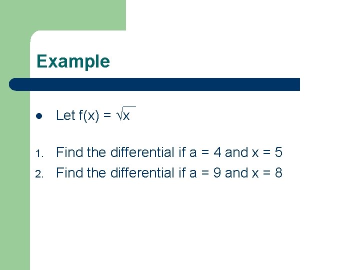
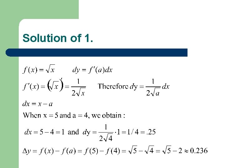
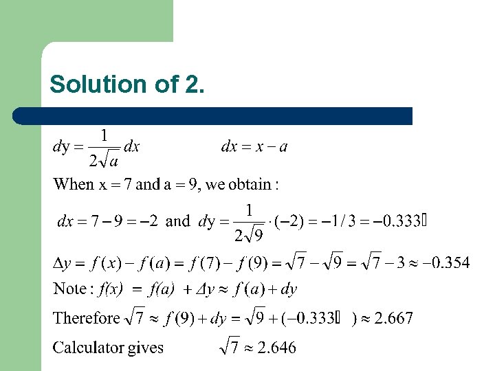
Example l Let f(x) = √x 1. Find the differential if a = 4 and x = 5 Find the differential if a = 9 and x = 8 2.

Solution of 1.

Solution of 2.

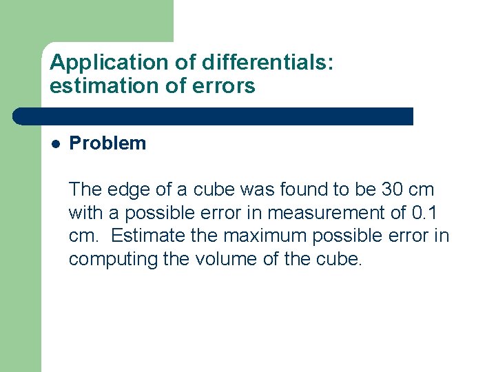
Application of differentials: estimation of errors l Problem The edge of a cube was found to be 30 cm with a possible error in measurement of 0. 1 cm. Estimate the maximum possible error in computing the volume of the cube.

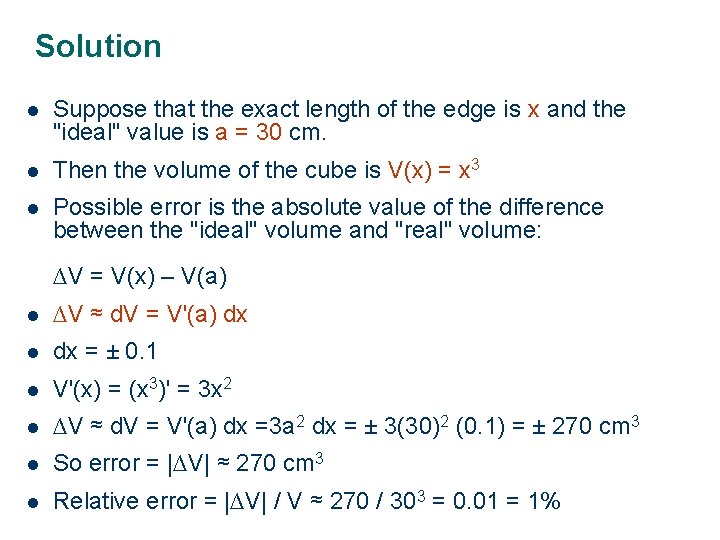
Solution l Suppose that the exact length of the edge is x and the "ideal" value is a = 30 cm. l Then the volume of the cube is V(x) = x 3 l Possible error is the absolute value of the difference between the "ideal" volume and "real" volume: ∆V = V(x) – V(a) l ∆V ≈ d. V = V'(a) dx l dx = ± 0. 1 l V'(x) = (x 3)' = 3 x 2 l ∆V ≈ d. V = V'(a) dx =3 a 2 dx = ± 3(30)2 (0. 1) = ± 270 cm 3 l So error = |∆V| ≈ 270 cm 3 l Relative error = |∆V| / V ≈ 270 / 303 = 0. 01 = 1%