Approximation Algorithms Pasi Frnti 16 9 2020 Approximation

Approximation Algorithms Pasi Fränti 16. 9. 2020

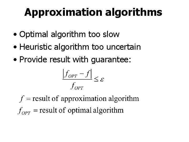
Approximation algorithms • Optimal algorithm too slow • Heuristic algorithm too uncertain • Provide result with guarantee:

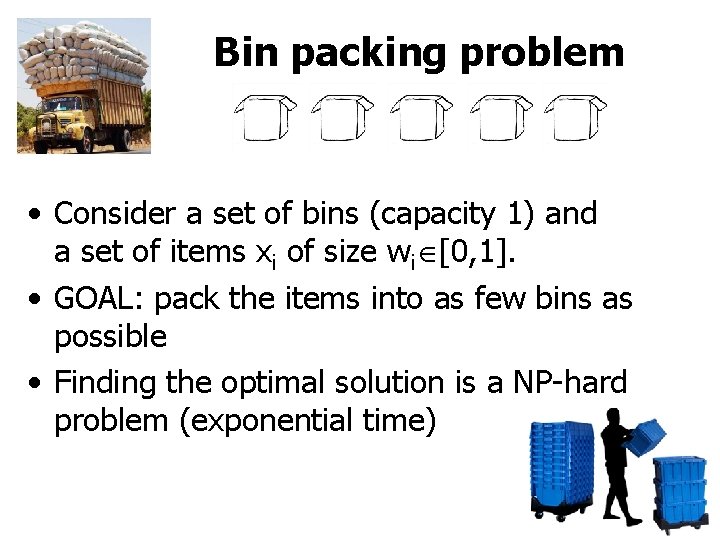
Bin packing problem • Consider a set of bins (capacity 1) and a set of items xi of size wi [0, 1]. • GOAL: pack the items into as few bins as possible • Finding the optimal solution is a NP-hard problem (exponential time)

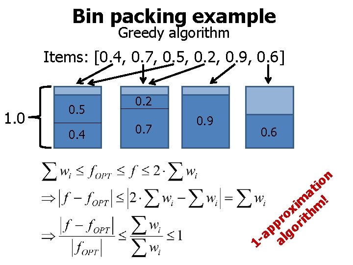
Bin packing example Greedy algorithm Items: [0. 4, 0. 7, 0. 5, 0. 2, 0. 9, 0. 6] 1. 0 0. 5 0. 4 0. 2 0. 7 0. 9 0. 6 n o i t a ! m m i x h o t r i r p o p a lg a 1

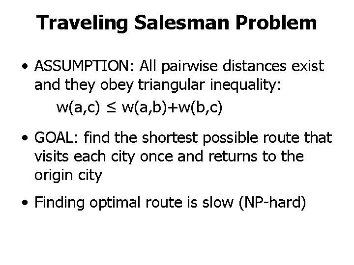
Traveling Salesman Problem • ASSUMPTION: All pairwise distances exist and they obey triangular inequality: w(a, c) ≤ w(a, b)+w(b, c) • GOAL: find the shortest possible route that visits each city once and returns to the origin city • Finding optimal route is slow (NP-hard)

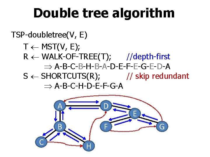
Double tree algorithm TSP-doubletree(V, E) T MST(V, E); R WALK-OF-TREE(T); //depth-first A-B-C-B-H-B-A-D-E-F-E-G-E-D-A S SHORTCUTS(R); // skip redundant A-B-C-H-D-E-F-G-A C A D B F H E G

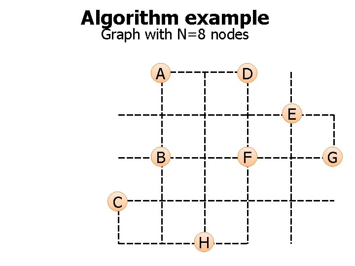
Algorithm example Graph with N=8 nodes A D E B F C H G

Algorithm example Minimum spanning tree 2 A 11. 9 D 2 2 B F 2 C 5 H 2 E 2 G

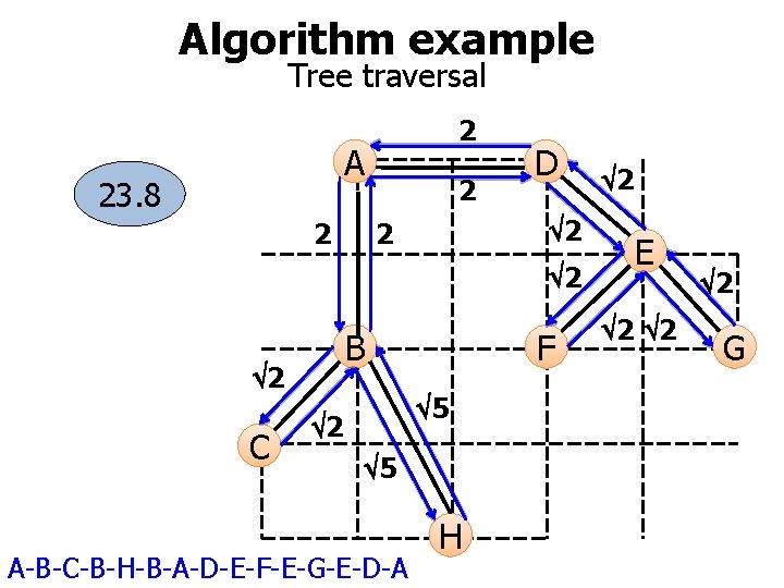
Algorithm example Tree traversal 2 A 23. 8 2 2 D 2 2 2 B 2 C F 5 2 5 A-B-C-B-H-B-A-D-E-F-E-G-E-D-A H 2 E 2 2 2 G

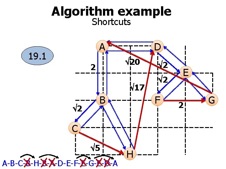
Algorithm example Shortcuts A 19. 1 D 20 2 17 2 B A-B-C-B-H-B-A-D-E-F-E-G-E-D-A 2 F C 5 2 H E 2 G

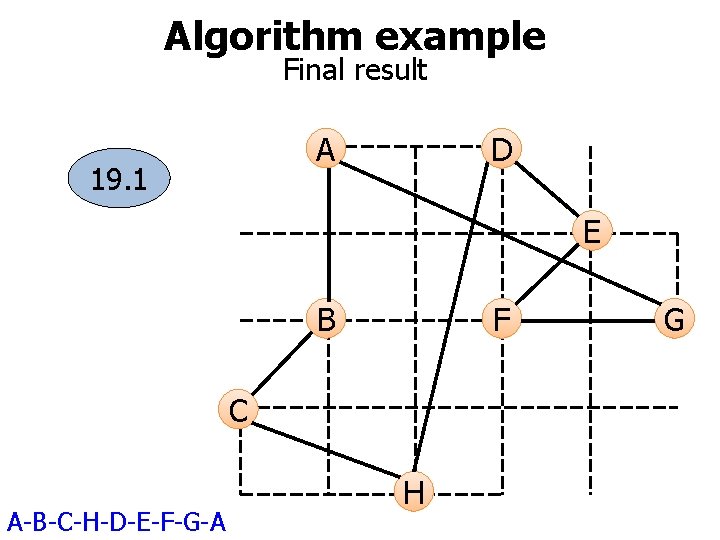
Algorithm example Final result A 19. 1 D E B F C A-B-C-H-D-E-F-G-A H G

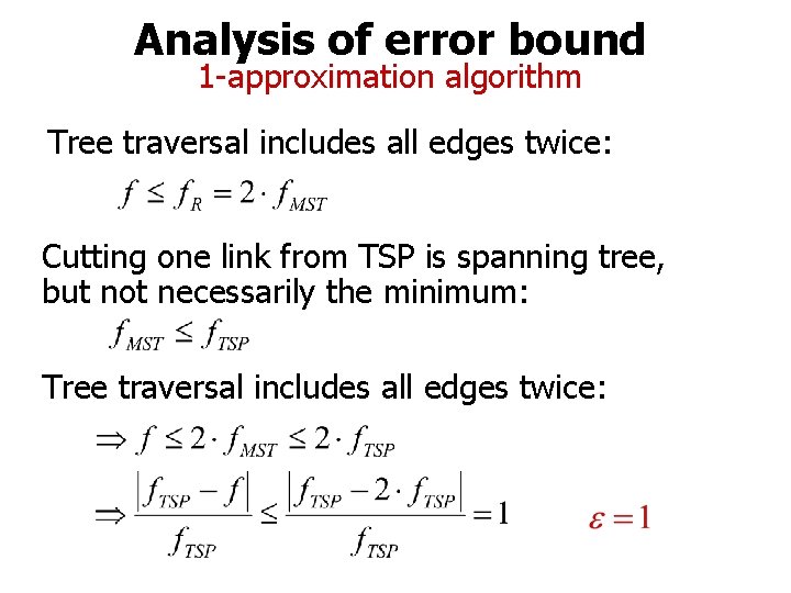
Analysis of error bound 1 -approximation algorithm Tree traversal includes all edges twice: Cutting one link from TSP is spanning tree, but not necessarily the minimum: Tree traversal includes all edges twice:

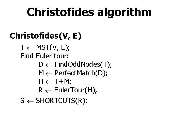
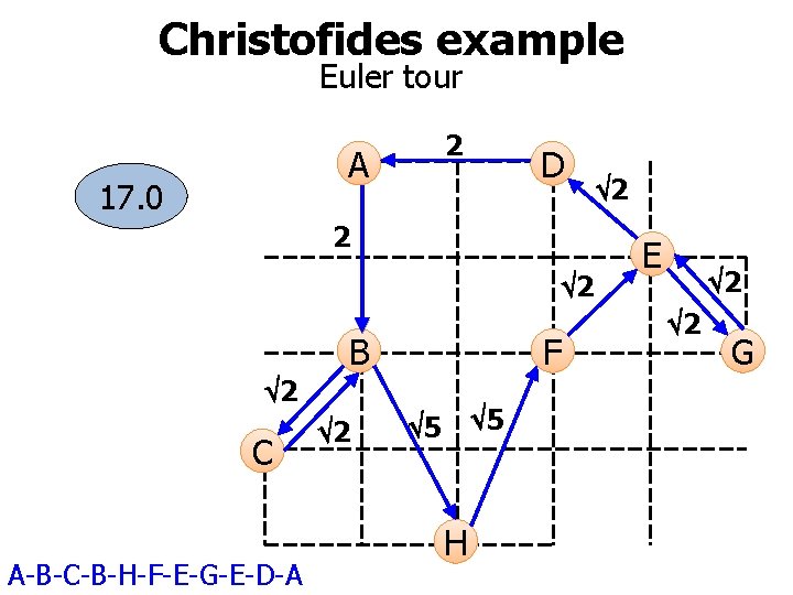
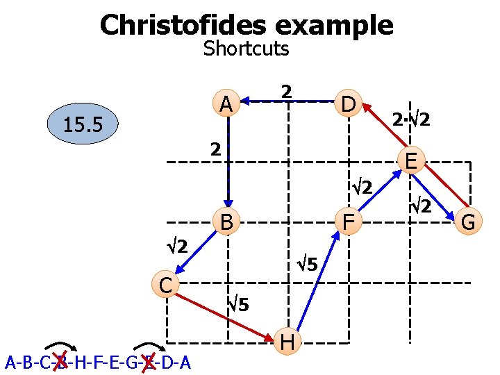
Christofides algorithm Christofides(V, E) T MST(V, E); Find Euler tour: D Find. Odd. Nodes(T); M Perfect. Match(D); H T+M; R Euler. Tour(H); S SHORTCUTS(R);

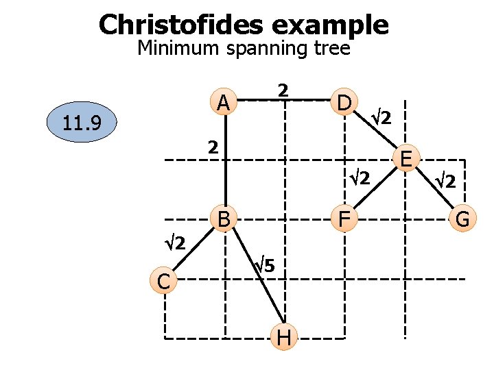
Christofides example Minimum spanning tree 2 A 11. 9 D 2 2 B F 2 C 5 H 2 E 2 G

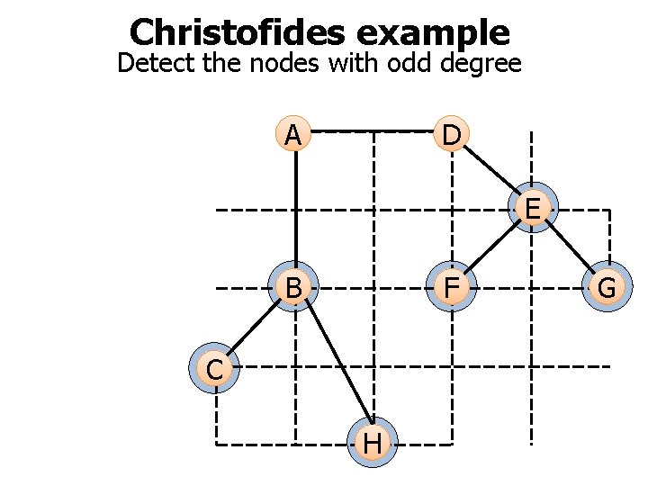
Christofides example Detect the nodes with odd degree A D E B F C H G

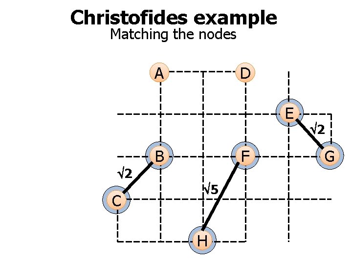
Christofides example Matching the nodes A D E B F 2 C 5 H 2 G

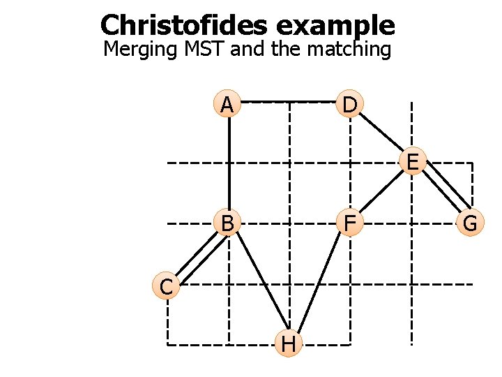
Christofides example Merging MST and the matching A D E B F C H G

Christofides example Euler tour A 17. 0 2 D 2 2 B 2 C A-B-C-B-H-F-E-G-E-D-A 2 F 5 5 H 2 E 2 2 G

Christofides example Shortcuts A 15. 5 2 D 2 E 2 B F 2 C A-B-C-B-H-F-E-G-E-D-A 2∙ 2 5 5 H 2 G

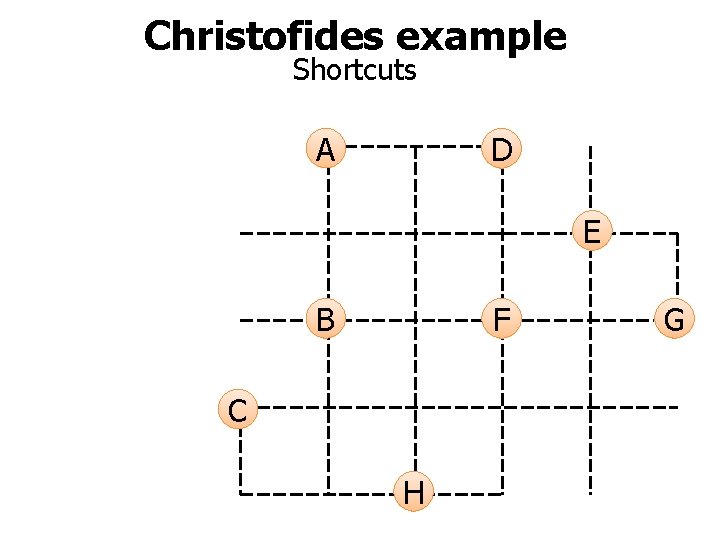
Christofides example Shortcuts A D E B F C H G

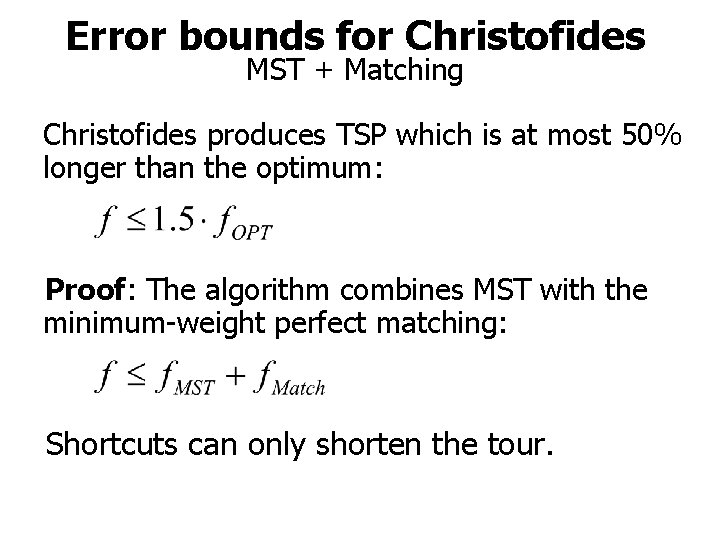
Error bounds for Christofides MST + Matching Christofides produces TSP which is at most 50% longer than the optimum: Proof: The algorithm combines MST with the minimum-weight perfect matching: Shortcuts can only shorten the tour.

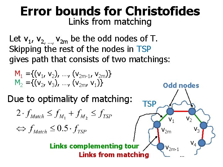
Error bounds for Christofides Links from matching Let v 1, v 2, …, v 2 m be the odd nodes of T. Skipping the rest of the nodes in TSP gives path that consists of two matchings: M 1 ={(v 1, v 2), …, (v 2 m-1, v 2 m)} M 2 ={(v 2, v 3), …, (v 2 m, v 1)} Due to optimality of matching: Odd nodes TSP v 2 v 1 v 3 v 2 m Links complementing tour Links from matching v 2 m-1 v 4 …

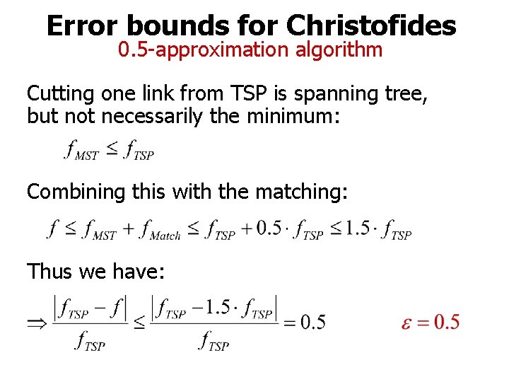
Error bounds for Christofides 0. 5 -approximation algorithm Cutting one link from TSP is spanning tree, but not necessarily the minimum: Combining this with the matching: Thus we have:

Empty space for notes

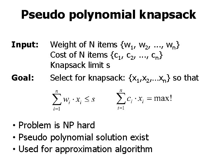
Pseudo polynomial knapsack Input: Goal: Weight of N items {w 1, w 2, . . . , wn} Cost of N items {c 1, c 2, . . . , cn} Knapsack limit s Select for knapsack: {x 1, x 2, …xn} so that • Problem is NP hard • Pseudo polynomial solution exist • Used for approximation algorithm

Pseudo polynomial knapsack Dynamic programming algorithm KNAPSACK (c[1, n], w[1, n], s} RETURNS x[1, n] w y Ne mb co If same cost prune R {(∅, 0)} Include if out weaker solution item fits in FOR i 1 TO n DO FOR (S, c) R DO IF Σj S wj+wi ≤ s THEN R R∪{(S∪{i}, c+ci)} FOR (S, c), (S’, c) R DO IF Σj S wj ≤ Σj S’ wj THEN R R{(S’, c)} ELSE R R{(S, c)} (S, c) (S, c’) R for which c’ is max! FOR i 1 TO n DO IF i S THEN x[i] 1 ELSE x[i] 0 RETURN x;

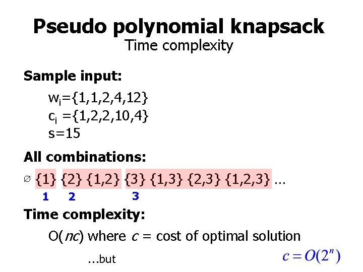
Pseudo polynomial knapsack Time complexity Sample input: wi={1, 1, 2, 4, 12} ci ={1, 2, 2, 10, 4} s=15 All combinations: ∅ {1} {2} {1, 2} {3} {1, 3} {2, 3} {1, 2, 3} … 1 3 2 Time complexity: O(nc) where c = cost of optimal solution …but

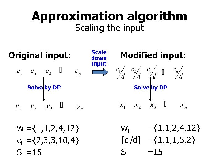
Approximation algorithm Scaling the input Original input: Solve by DP wi ={1, 1, 2, 4, 12} ci ={2, 3, 3, 10, 4} S =15 Scale down input Modified input: Solve by DP wi ={1, 1, 2, 4, 12} [ci/d] ={1, 1, 1, 5, 2} S =15

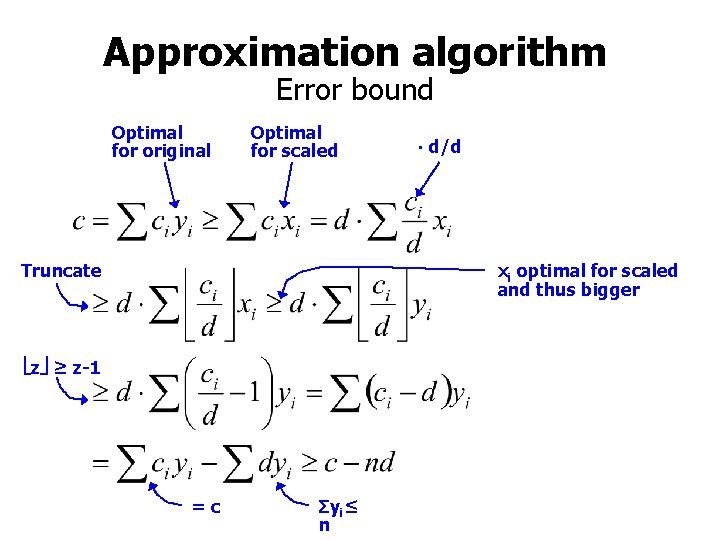
Approximation algorithm Error bound Optimal for original Optimal for scaled Truncate ∙ d/d xi optimal for scaled and thus bigger z ≥ z-1 =c Σyi≤ n

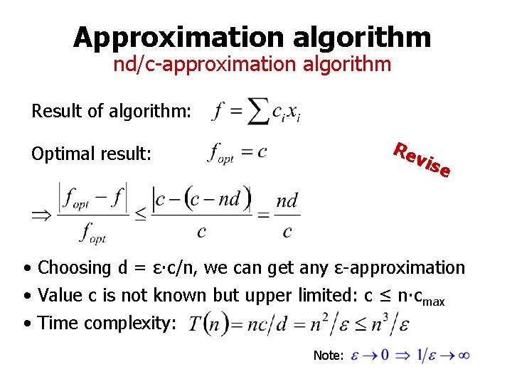
Approximation algorithm nd/c-approximation algorithm Result of algorithm: Re Optimal result: vis e • Choosing d = ε∙c/n, we can get any ε-approximation • Value c is not known but upper limited: c ≤ n∙cmax • Time complexity: Note:

Empty space for notes 1 A 4 B 2 3 E 3 ? C F 4 1 D

Acknowledgements Contributions by Sharon Guardado and Pekka T. Kilpeläinen to TSP example and its proof appreciated.