Mathematical Programming especially Integer Linear Programming and Mixed

Mathematical Programming especially Integer Linear Programming and Mixed Integer Programming 600. 325/425 Declarative Methods - J. Eisner 1

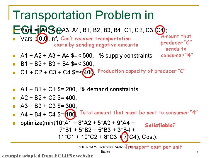
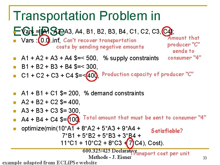
Transportation Problem in Vars = [A 1, A 2, A 3, A 4, B 1, B 2, B 3, B 4, C 1, C 2, C 3, C 4]; ECLi. PSe Amount that n n n n n Vars : : 0. 0. . inf, Can’t recover transportation costs by sending negative amounts producer “C” sends to consumer “ 4” A 1 + A 2 + A 3 + A 4 $=< 500, % supply constraints B 1 + B 2 + B 3 + B 4 $=< 300, C 1 + C 2 + C 3 + C 4 $=< 400, Production capacity of producer “C” A 1 + B 1 + C 1 $= 200, % demand constraints A 2 + B 2 + C 2 $= 400, A 3 + B 3 + C 3 $= 300, A 4 + B 4 + C 4 $= 100, Total amount that must be sent to consumer “ 4” optimize(min(10*A 1 + 8*A 2 + 5*A 3 + 9*A 4 + Satisfiable? 7*B 1 + 5*B 2 + 5*B 3 + 3*B 4 + 11*C 1 + 10*C 2 + 8*C 3 + 7*C 4), Cost). 600. 325/425 Declarative Methods - J. Transport Eisner example adapted from ECLi. PSe website cost per unit 2

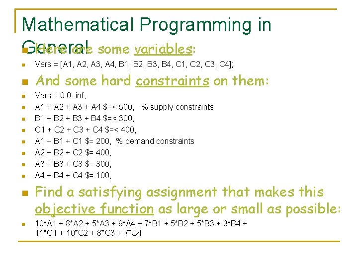
Mathematical Programming in General n Here are some variables: n Vars = [A 1, A 2, A 3, A 4, B 1, B 2, B 3, B 4, C 1, C 2, C 3, C 4]; n And some hard constraints on them: n n n n n Vars : : 0. 0. . inf, A 1 + A 2 + A 3 + A 4 $=< 500, % supply constraints B 1 + B 2 + B 3 + B 4 $=< 300, C 1 + C 2 + C 3 + C 4 $=< 400, A 1 + B 1 + C 1 $= 200, % demand constraints A 2 + B 2 + C 2 $= 400, A 3 + B 3 + C 3 $= 300, A 4 + B 4 + C 4 $= 100, Find a satisfying assignment that makes this objective function as large or small as possible: 10*A 1 + 8*A 2 + 5*A 3 + 9*A 4 + 7*B 1 + 5*B 2 + 5*B 3 + 3*B 4 + 11*C 1 + 10*C 2 + 8*C 3 + 7*C 4

Mathematical Programming in General n Here are some variables: n n And some hard constraints on them: Find a satisfying assignment that makes this objective function as large or small as possible:

Types of Mathematical Programming

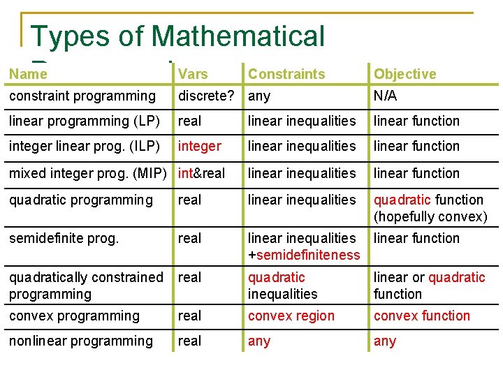
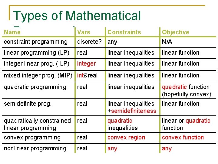
Types of Mathematical Name Vars Constraints Programming Objective constraint programming discrete? any N/A linear programming (LP) real linear inequalities linear function integer linear prog. (ILP) integer linear inequalities linear function mixed integer prog. (MIP) int&real linear inequalities linear function quadratic programming real linear inequalities quadratic function (hopefully convex) semidefinite prog. real linear inequalities linear function +semidefiniteness quadratically constrained programming real quadratic inequalities linear or quadratic function convex programming real convex region convex function nonlinear programming real any

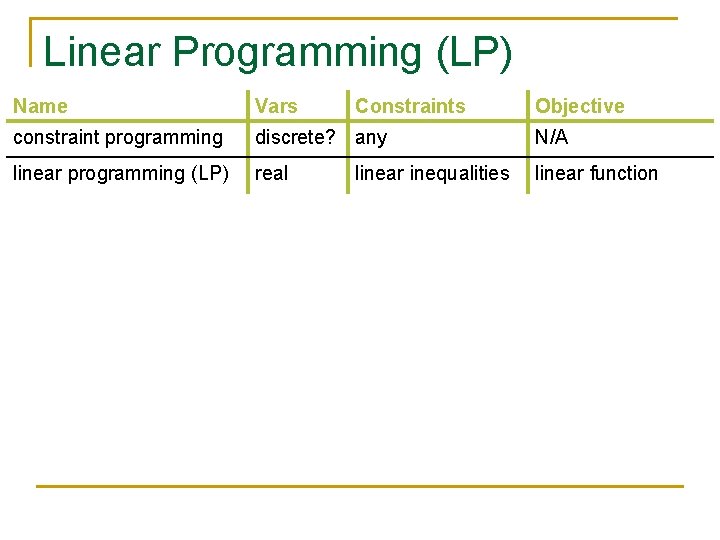
Linear Programming (LP) Name Vars Constraints constraint programming discrete? any N/A linear programming (LP) real linear function linear inequalities Objective

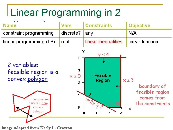
Linear Programming in 2 Name dimensions. Vars Constraints Objective constraint programming discrete? any N/A linear programming (LP) real linear function linear inequalities y 4 2 variables: feasible region is a convex polygon x 0 for comparison, here’s a nonconvex polygon image adapted from Keely L. Croxton x 3 x+ 2 y 2 y 0 boundary of feasible region comes from the constraints

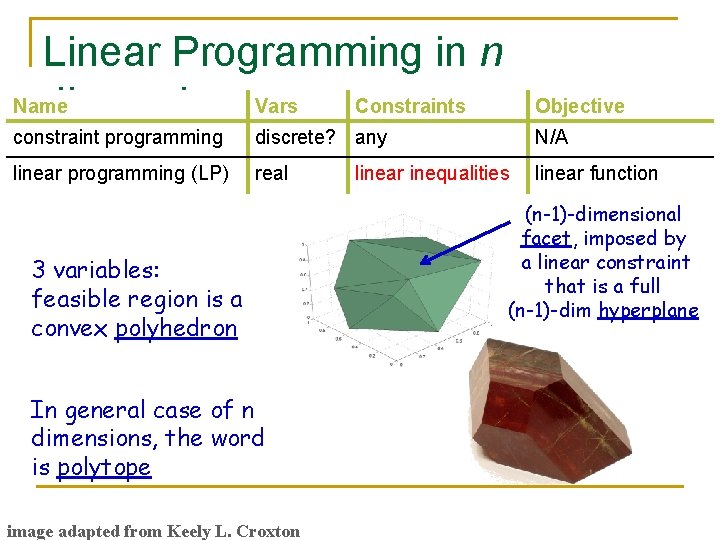
Linear Programming in n Name dimensions. Vars Constraints Objective constraint programming discrete? any N/A linear programming (LP) real linear function 3 variables: feasible region is a convex polyhedron In general case of n dimensions, the word is polytope image adapted from Keely L. Croxton linear inequalities (n-1)-dimensional facet, imposed by a linear constraint that is a full (n-1)-dim hyperplane

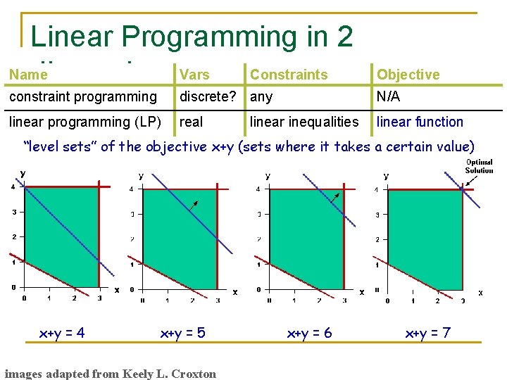
Linear Programming in 2 Name dimensions. Vars Constraints Objective constraint programming discrete? any N/A linear programming (LP) real linear function linear inequalities “level sets” of the objective x+y (sets where it takes a certain value) x+y = 4 x+y = 5 images adapted from Keely L. Croxton x+y = 6 x+y = 7

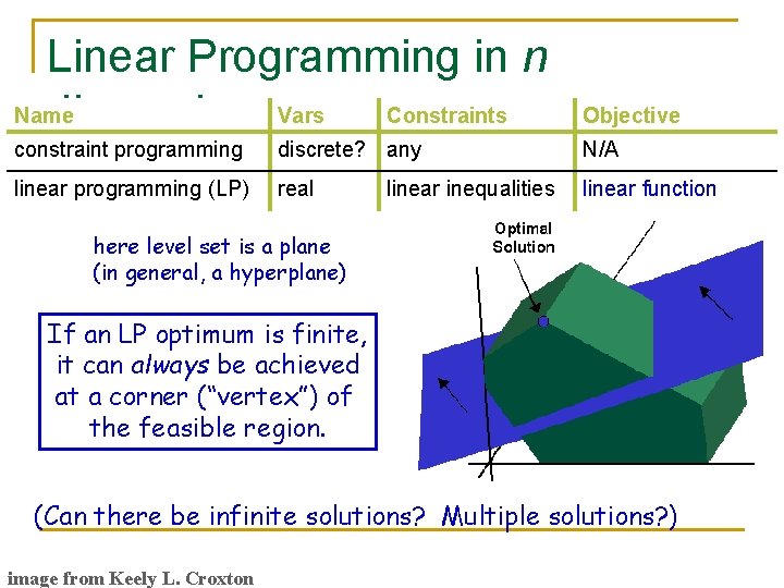
Linear Programming in n Name dimensions. Vars Constraints Objective constraint programming discrete? any N/A linear programming (LP) real linear function linear inequalities here level set is a plane (in general, a hyperplane) If an LP optimum is finite, it can always be achieved at a corner (“vertex”) of the feasible region. (Can there be infinite solutions? Multiple solutions? ) image from Keely L. Croxton

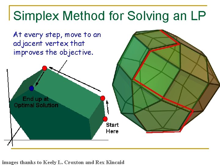
Simplex Method for Solving an LP At every step, move to an adjacent vertex that improves the objective. images thanks to Keely L. Croxton and Rex Kincaid

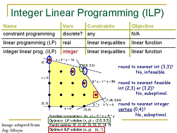
Integer Linear Programming (ILP) Name Vars Constraints Objective constraint programming discrete? any N/A linear programming (LP) real linear inequalities linear function integer linear prog. (ILP) integer linear inequalities linear function round to nearest int (3, 3)? No, infeasible. round to nearest feasible int (2, 3) or (3, 2)? No, suboptimal. round to nearest integer vertex (0, 4)? No, suboptimal. image adapted from Jop Sibeyn

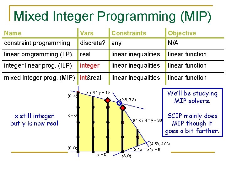
Mixed Integer Programming (MIP) Name Vars constraint programming discrete? any N/A linear programming (LP) real linear inequalities linear function integer linear prog. (ILP) integer linear inequalities linear function mixed integer prog. (MIP) int&real Constraints Objective We’ll be studying MIP solvers. x still integer but y is now real SCIP mainly does MIP though it goes a bit farther.

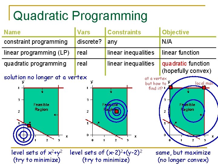
Quadratic Programming Name Vars Constraints constraint programming discrete? any N/A linear programming (LP) real linear inequalities linear function quadratic programming real linear inequalities quadratic function (hopefully convex) solution no longer at a vertex level sets of x 2+y 2 (try to minimize) level sets of (x-2)2+(y-2)2 (try to minimize) Objective at a vertex but how to find it? local max same, but maximize (no longer convex)

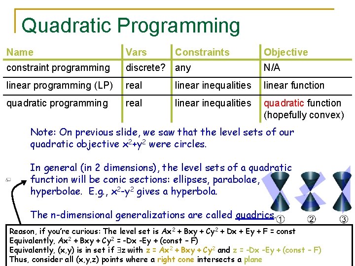
Quadratic Programming Name Vars Constraints Objective constraint programming discrete? any N/A linear programming (LP) real linear inequalities linear function quadratic programming real linear inequalities quadratic function (hopefully convex) Note: On previous slide, we saw that the level sets of our quadratic objective x 2+y 2 were circles. In general (in 2 dimensions), the level sets of a quadratic function will be conic sections: ellipses, parabolae, hyperbolae. E. g. , x 2 -y 2 gives a hyperbola. The n-dimensional generalizations are called quadrics. Reason, if you’re curious: The level set is Ax 2 + Bxy + Cy 2 + Dx + Ey + F = const Equivalently, Ax 2 + Bxy + Cy 2 = -Dx -Ey + (const – F) Equivalently, (x, y) is in set if z with z = Ax 2 + Bxy + Cy 2 and z = -Dx -Ey + (const – F) Thus, consider all (x, y, z) points where a right cone intersects a plane

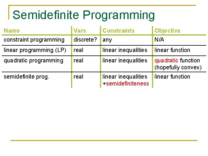
Semidefinite Programming Name Vars Constraints Objective constraint programming discrete? any N/A linear programming (LP) real linear inequalities linear function quadratic programming real linear inequalities quadratic function (hopefully convex) semidefinite prog. real linear inequalities linear function +semidefiniteness

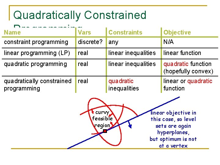
Quadratically Constrained Programming. Vars Constraints Name Objective constraint programming discrete? any N/A linear programming (LP) real linear inequalities linear function quadratic programming real linear inequalities quadratic function (hopefully convex) quadratically constrained programming real quadratic inequalities linear or quadratic function curvy feasible region linear objective in this case, so level sets are again hyperplanes, but optimum is not at a vertex

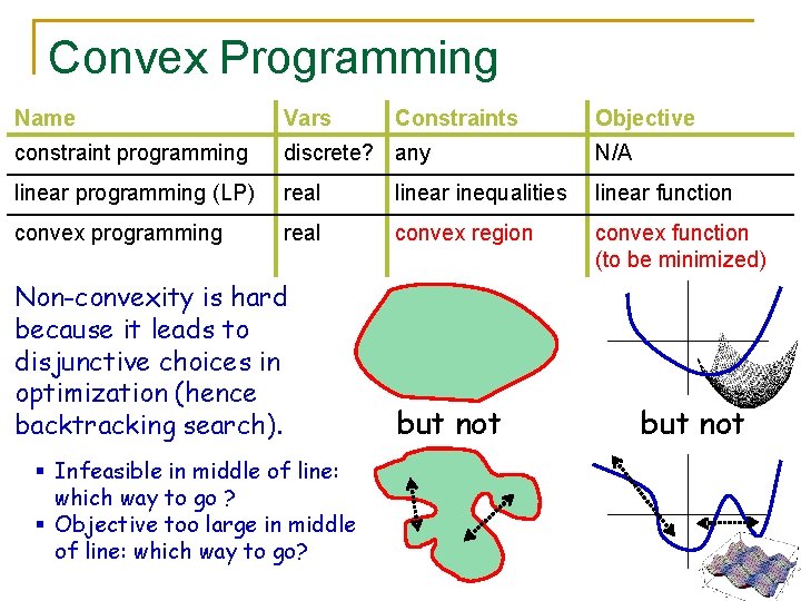
Convex Programming Name Vars constraint programming discrete? any N/A linear programming (LP) real linear inequalities linear function convex programming real convex region convex function (to be minimized) Non-convexity is hard because it leads to disjunctive choices in optimization (hence backtracking search). § Infeasible in middle of line: which way to go ? § Objective too large in middle of line: which way to go? Constraints but not Objective but not

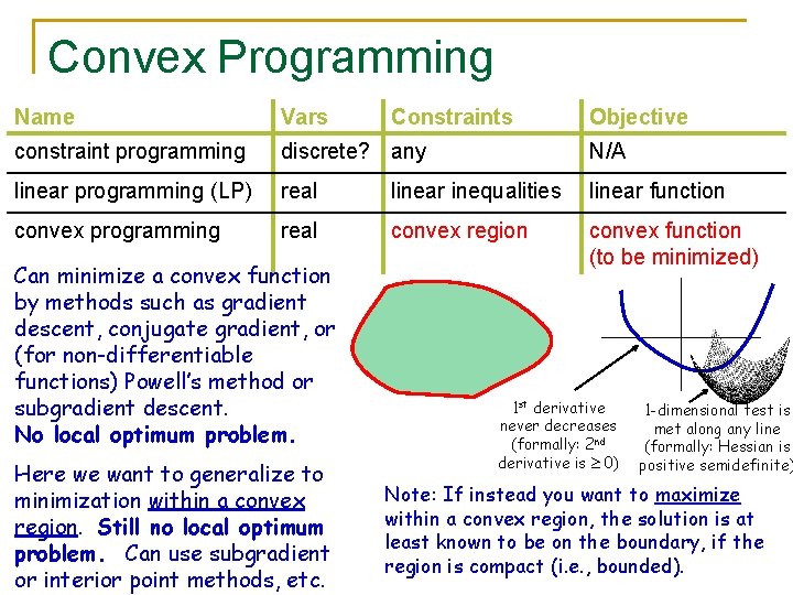
Convex Programming Name Vars constraint programming discrete? any N/A linear programming (LP) real linear inequalities linear function convex programming real convex region convex function (to be minimized) Can minimize a convex function by methods such as gradient descent, conjugate gradient, or (for non-differentiable functions) Powell’s method or subgradient descent. No local optimum problem. Here we want to generalize to minimization within a convex region. Still no local optimum problem. Can use subgradient or interior point methods, etc. Constraints Objective 1 st derivative never decreases (formally: 2 nd derivative is 0) 1 -dimensional test is met along any line (formally: Hessian is positive semidefinite) Note: If instead you want to maximize within a convex region, the solution is at least known to be on the boundary, if the region is compact (i. e. , bounded).

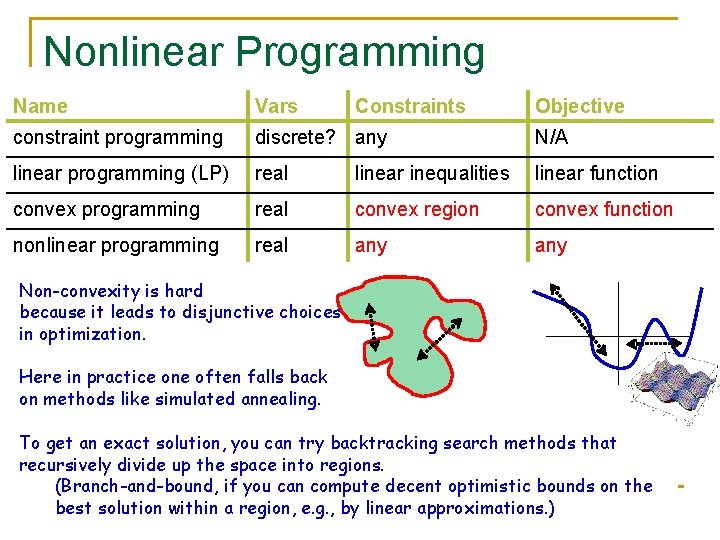
Nonlinear Programming Name Vars Constraints Objective constraint programming discrete? any N/A linear programming (LP) real linear inequalities linear function convex programming real convex region convex function nonlinear programming real any Non-convexity is hard because it leads to disjunctive choices in optimization. Here in practice one often falls back on methods like simulated annealing. To get an exact solution, you can try backtracking search methods that recursively divide up the space into regions. (Branch-and-bound, if you can compute decent optimistic bounds on the best solution within a region, e. g. , by linear approximations. )

Types of Mathematical Name Vars Constraints Programming Objective constraint programming discrete? any N/A linear programming (LP) real linear inequalities linear function integer linear prog. (ILP) integer linear inequalities linear function mixed integer prog. (MIP) int&real linear inequalities linear function quadratic programming real linear inequalities quadratic function (hopefully convex) semidefinite prog. real linear inequalities linear function +semidefiniteness quadratically constrained linear programming real quadratic inequalities linear or quadratic function convex programming real convex region convex function nonlinear programming real any

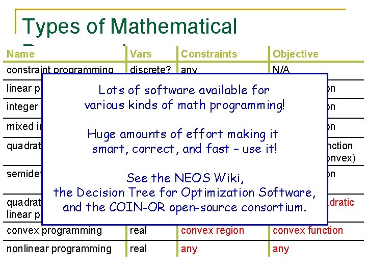
Types of Mathematical Name Vars Constraints Programming Objective constraint programming N/A discrete? any linear programming (LP) realsoftware linear inequalities Lots of available for linear function various programming! integer linear prog. (ILP) kinds integerof math linear inequalities linear function mixed integer prog. (MIP) int&real linear inequalities linear function Huge amounts of effort making it quadratic programming inequalities smart, real correct, linear and fast – use it!quadratic function (hopefully convex) semidefinite prog. real the NEOS linear inequalities linear function See Wiki, +semidefiniteness the Decision Tree for Optimization Software, quadratically constrained real quadratic linear or quadratic and the COIN-OR open-source consortium. linear programming inequalities function convex programming real convex region convex function nonlinear programming real any

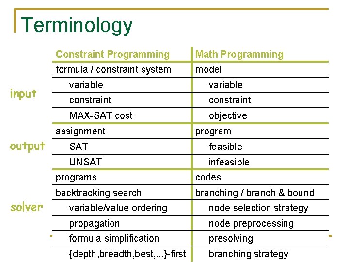
Terminology input Constraint Programming Math Programming formula / constraint system model variable constraint MAX-SAT cost objective assignment output solver program SAT feasible UNSAT infeasible programs codes backtracking search branching / branch & bound variable/value ordering node selection strategy propagation node preprocessing formula simplification presolving {depth, breadth, best, . . . }-first branching strategy

Linear Programming in ZIMPL

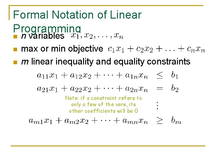
Formal Notation of Linear Programming n n variables max or min objective m linear inequality and equality constraints Note: if a constraint refers to only a few of the vars, its other coefficients will be 0

Formal Notation of Linear Programming n n variables max or min objective m linear inequality and equality constraints Note: if a constraint refers to only a few of the vars, its other coefficients will be 0

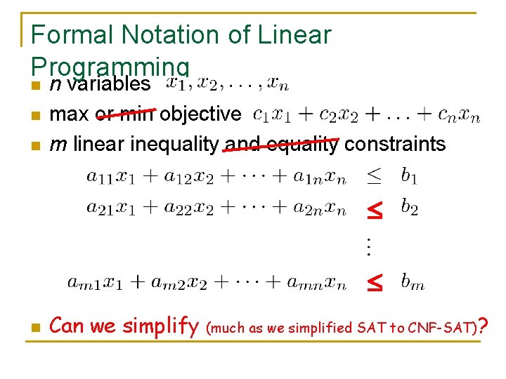
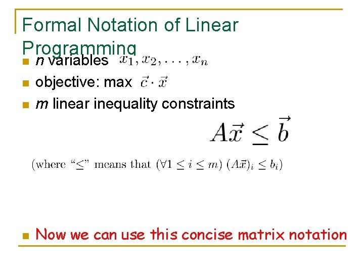
Formal Notation of Linear Programming n n variables max or min objective m linear inequality and equality constraints n Can we simplify (much as we simplified SAT to CNF-SAT)?

Formal Notation of Linear Programming n n variables objective: max m linear inequality constraints n Now we can use this concise matrix notation n n

Formal Notation of Linear Programming n n variables objective: max m linear inequality constraints n Some LP folks also assume constraint n n q q What if you want to allow x 3 < 0? Just replace x 3 everywhere with (xn+1 - xn+2) where xn+1, xn+2 are new variables 0. Then solver can pick xn+1, xn+2 to have either pos or neg diff.

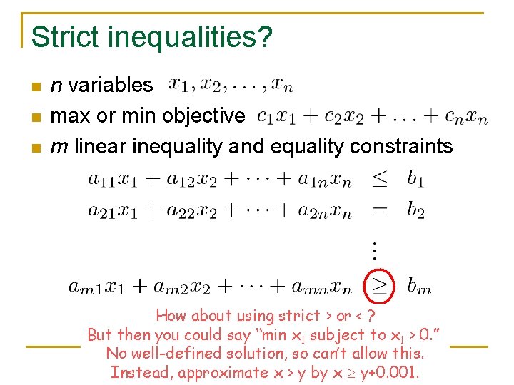
Strict inequalities? n n variables max or min objective m linear inequality and equality constraints How about using strict > or < ? But then you could say “min x 1 subject to x 1 > 0. ” No well-defined solution, so can’t allow this. Instead, approximate x > y by x y+0. 001.

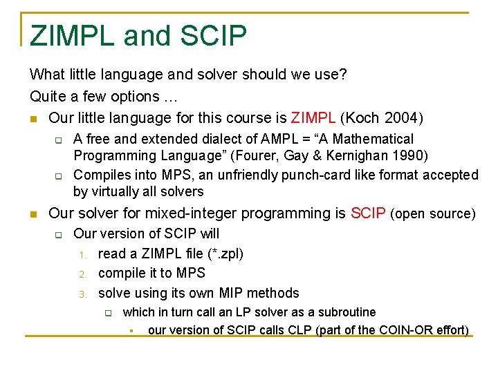
ZIMPL and SCIP What little language and solver should we use? Quite a few options … n Our little language for this course is ZIMPL (Koch 2004) q q n A free and extended dialect of AMPL = “A Mathematical Programming Language” (Fourer, Gay & Kernighan 1990) Compiles into MPS, an unfriendly punch-card like format accepted by virtually all solvers Our solver for mixed-integer programming is SCIP (open source) q Our version of SCIP will 1. read a ZIMPL file (*. zpl) 2. compile it to MPS 3. solve using its own MIP methods q which in turn call an LP solver as a subroutine § our version of SCIP calls CLP (part of the COIN-OR effort)

Transportation Problem in Vars = [A 1, A 2, A 3, A 4, B 1, B 2, B 3, B 4, C 1, C 2, C 3, C 4]; ECLi. PSe Amount that n n n n n Vars : : 0. 0. . inf, Can’t recover transportation costs by sending negative amounts producer “C” sends to consumer “ 4” A 1 + A 2 + A 3 + A 4 $=< 500, % supply constraints B 1 + B 2 + B 3 + B 4 $=< 300, C 1 + C 2 + C 3 + C 4 $=< 400, Production capacity of producer “C” A 1 + B 1 + C 1 $= 200, % demand constraints A 2 + B 2 + C 2 $= 400, A 3 + B 3 + C 3 $= 300, A 4 + B 4 + C 4 $= 100, Total amount that must be sent to consumer “ 4” optimize(min(10*A 1 + 8*A 2 + 5*A 3 + 9*A 4 + Satisfiable? 7*B 1 + 5*B 2 + 5*B 3 + 3*B 4 + 11*C 1 + 10*C 2 + 8*C 3 + 7*C 4), Cost). 600. 325/425 Declarative Transport cost per unit Methods - J. Eisner example adapted from ECLi. PSe website 33

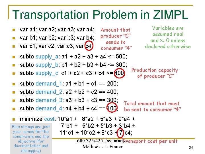
Transportation Problem in ZIMPL n n n n n var a 1; var a 2; var a 3; var a 4; var b 1; var b 2; var b 3; var b 4; var c 1; var c 2; var c 3; var c 4; Amount that producer “C” sends to consumer “ 4” Variables are assumed real and >= 0 unless declared otherwise subto supply_a: a 1 + a 2 + a 3 + a 4 <= 500; subto supply_b: b 1 + b 2 + b 3 + b 4 <= 300; Production capacity subto supply_c: c 1 + c 2 + c 3 + c 4 <= 400; of producer “C” subto demand_1: a 1 + b 1 + c 1 == 200; subto demand_2: a 2 + b 2 + c 2 == 400; subto demand_3: a 3 + b 3 + c 3 == 300; Total amount that must subto demand_4: a 4 + b 4 + c 4 == 100; be sent to consumer “ 4” minimize cost: 10*a 1 + 8*a 2 + 5*a 3 + 9*a 4 + 7*b 1 + 5*b 2 + 5*b 3 + 3*b 4 + Blue strings are just your names for the 11*c 1 + 10*c 2 + 8*c 3 + 7*c 4; n constraints and the objective (for documentation and debugging) 600. 325/425 Declarative Transport cost per unit Methods - J. Eisner 34

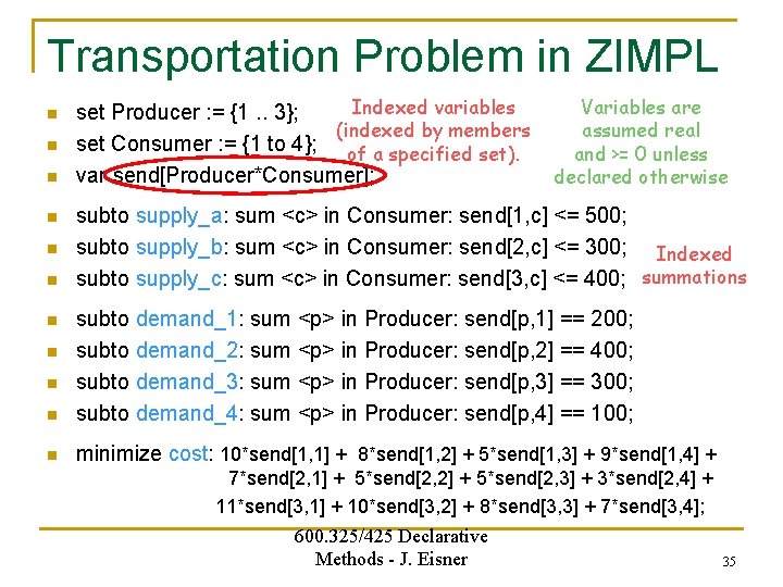
Transportation Problem in ZIMPL n n n Indexed variables set Producer : = {1. . 3}; (indexed by members set Consumer : = {1 to 4}; of a specified set). var send[Producer*Consumer]; Variables are assumed real and >= 0 unless declared otherwise subto supply_a: sum <c> in Consumer: send[1, c] <= 500; subto supply_b: sum <c> in Consumer: send[2, c] <= 300; Indexed subto supply_c: sum <c> in Consumer: send[3, c] <= 400; summations n subto demand_1: sum <p> in Producer: send[p, 1] == 200; subto demand_2: sum <p> in Producer: send[p, 2] == 400; subto demand_3: sum <p> in Producer: send[p, 3] == 300; subto demand_4: sum <p> in Producer: send[p, 4] == 100; n minimize cost: 10*send[1, 1] + 8*send[1, 2] + 5*send[1, 3] + 9*send[1, 4] + n n n 7*send[2, 1] + 5*send[2, 2] + 5*send[2, 3] + 3*send[2, 4] + 11*send[3, 1] + 10*send[3, 2] + 8*send[3, 3] + 7*send[3, 4]; 600. 325/425 Declarative Methods - J. Eisner 35

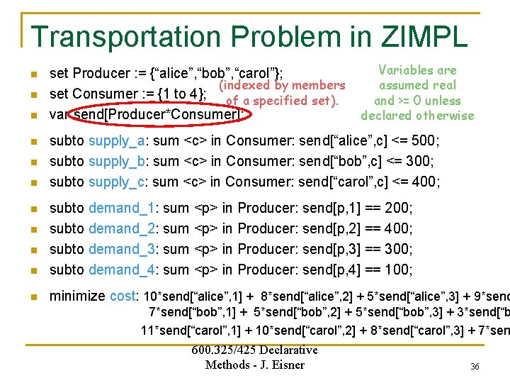
Transportation Problem in ZIMPL n n n set Producer : = {“alice”, “bob”, “carol”}; (indexed by members set Consumer : = {1 to 4}; of a specified set). var send[Producer*Consumer]; Variables are assumed real and >= 0 unless declared otherwise subto supply_a: sum <c> in Consumer: send[“alice”, c] <= 500; subto supply_b: sum <c> in Consumer: send[“bob”, c] <= 300; subto supply_c: sum <c> in Consumer: send[“carol”, c] <= 400; n subto demand_1: sum <p> in Producer: send[p, 1] == 200; subto demand_2: sum <p> in Producer: send[p, 2] == 400; subto demand_3: sum <p> in Producer: send[p, 3] == 300; subto demand_4: sum <p> in Producer: send[p, 4] == 100; n minimize cost: 10*send[“alice”, 1] + 8*send[“alice”, 2] + 5*send[“alice”, 3] + 9*send n n n 7*send[“bob”, 1] + 5*send[“bob”, 2] + 5*send[“bob”, 3] + 3*send[“b 11*send[“carol”, 1] + 10*send[“carol”, 2] + 8*send[“carol”, 3] + 7*sen 600. 325/425 Declarative Methods - J. Eisner 36

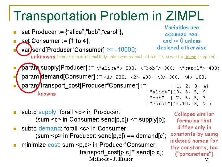
Transportation Problem in ZIMPL n n n set Producer : = {“alice”, “bob”, “carol”}; set Consumer : = {1 to 4}; var send[Producer*Consumer]; >= -10000; unknowns (remark: mustn’t multiply unknowns by each other if you want a linear program) param supply[Producer] : = <"alice"> 500, <"bob"> 300, <"carol"> 400; param demand[Consumer] : = <1> 200, <2> 400, <3> 300, <4> 100; param transport_cost[Producer*Consumer] : = | 1, 2, 3, 4| |"alice"|10, 8, 5, 9| |"bob" | 7, 5, 5, 3| |"carol"|11, 10, 8, 7|; knowns n n n Variables are assumed real and >= 0 unless declared otherwise subto supply: forall <p> in Producer: Collapse similar (sum <c> in Consumer: send[p, c]) <= supply[p]; formulas that differ only in subto demand: forall <c> in Consumer: (sum <p> in Producer: send[p, c]) == demand[c]; constants by using indexed names for minimize cost: sum <p, c> in Producer*Consumer: the constants, too 600. 325/425 Declarative transport_cost[p, c] * send[p, c]; (“parameters”) Methods - J. Eisner 37

How to Encode Interesting Things in LP (sometimes needs MIP)

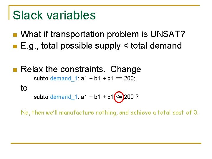
Slack variables n What if transportation problem is UNSAT? E. g. , total possible supply < total demand n Relax the constraints. Change n subto demand_1: a 1 + b 1 + c 1 == 200; to subto demand_1: a 1 + b 1 + c 1 <= 200 ? No, then we’ll manufacture nothing, and achieve a total cost of 0.

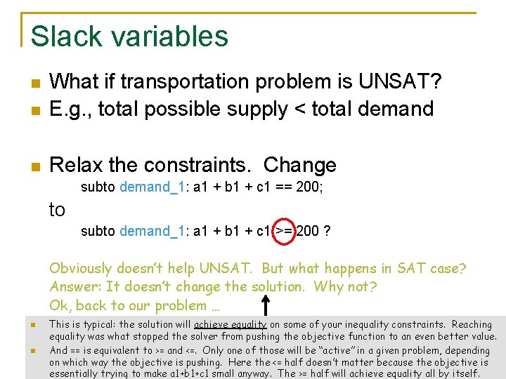
Slack variables n What if transportation problem is UNSAT? E. g. , total possible supply < total demand n Relax the constraints. Change n subto demand_1: a 1 + b 1 + c 1 == 200; to subto demand_1: a 1 + b 1 + c 1 >= 200 ? Obviously doesn’t help UNSAT. But what happens in SAT case? Answer: It doesn’t change the solution. Why not? Ok, back to our problem … n n This is typical: the solution will achieve equality on some of your inequality constraints. Reaching equality was what stopped the solver from pushing the objective function to an even better value. And == is equivalent to >= and <=. Only one of those will be “active” in a given problem, depending on which way the objective is pushing. Here the <= half doesn’t matter because the objective is essentially trying to make a 1+b 1+c 1 small anyway. The >= half will achieve equality all by itself.

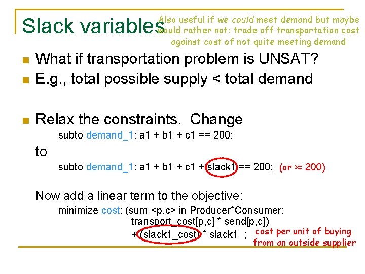
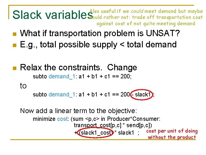
Also useful if we could meet demand but maybe would rather not: trade off transportation cost against cost of not quite meeting demand Slack variables n What if transportation problem is UNSAT? E. g. , total possible supply < total demand n Relax the constraints. Change n subto demand_1: a 1 + b 1 + c 1 == 200; to subto demand_1: a 1 + b 1 + c 1 + slack 1 == 200; (or >= 200) Now add a linear term to the objective: minimize cost: (sum <p, c> in Producer*Consumer: transport_cost[p, c] * send[p, c]) + (slack 1_cost) * slack 1 ; cost per unit of buying from an outside supplier

Also useful if we could meet demand but maybe would rather not: trade off transportation cost against cost of not quite meeting demand Slack variables n What if transportation problem is UNSAT? E. g. , total possible supply < total demand n Relax the constraints. Change n subto demand_1: a 1 + b 1 + c 1 == 200; to subto demand_1: a 1 + b 1 + c 1 == 200 - slack 1 ; Now add a linear term to the objective: minimize cost: (sum <p, c> in Producer*Consumer: transport_cost[p, c] * send[p, c]) + (slack 1_cost) * slack 1 ; cost per unit of doing without the product

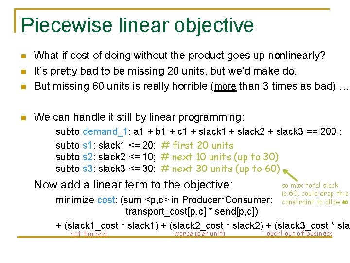
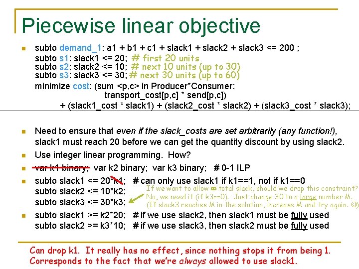
Piecewise linear objective n What if cost of doing without the product goes up nonlinearly? It’s pretty bad to be missing 20 units, but we’d make do. But missing 60 units is really horrible (more than 3 times as bad) … n We can handle it still by linear programming: n n subto demand_1: a 1 + b 1 + c 1 + slack 2 + slack 3 == 200 ; subto s 1: slack 1 <= 20; # first 20 units subto s 2: slack 2 <= 10; # next 10 units (up to 30) subto s 3: slack 3 <= 30; # next 30 units (up to 60) Now add a linear term to the objective: so max total slack is 60; could drop this constraint to allow minimize cost: (sum <p, c> in Producer*Consumer: transport_cost[p, c] * send[p, c]) + (slack 1_cost * slack 1) + (slack 2_cost * slack 2) + (slack 3_cost * sla not too bad worse (per unit) ouch! out of business

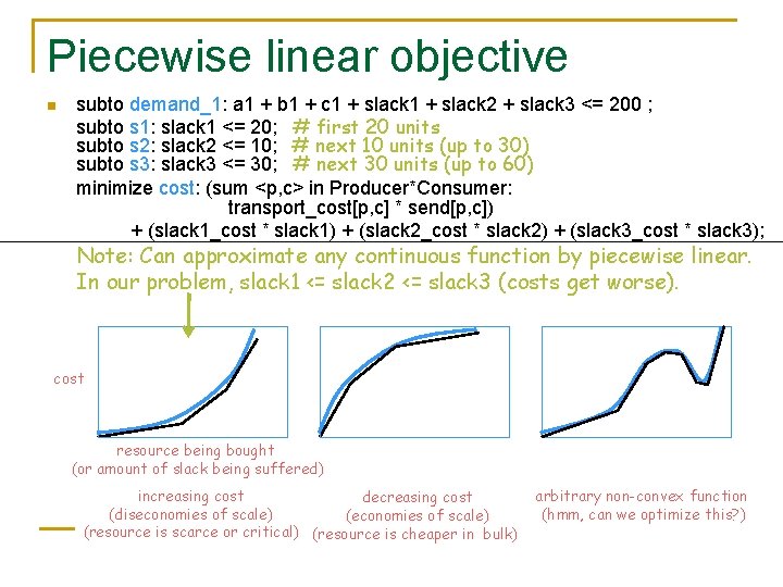
Piecewise linear objective n subto demand_1: a 1 + b 1 + c 1 + slack 2 + slack 3 <= 200 ; subto s 1: slack 1 <= 20; # first 20 units subto s 2: slack 2 <= 10; # next 10 units (up to 30) subto s 3: slack 3 <= 30; # next 30 units (up to 60) minimize cost: (sum <p, c> in Producer*Consumer: transport_cost[p, c] * send[p, c]) + (slack 1_cost * slack 1) + (slack 2_cost * slack 2) + (slack 3_cost * slack 3); Note: Can approximate any continuous function by piecewise linear. In our problem, slack 1 <= slack 2 <= slack 3 (costs get worse). cost resource being bought (or amount of slack being suffered) increasing cost decreasing cost (diseconomies of scale) (resource is scarce or critical) (resource is cheaper in bulk) arbitrary non-convex function (hmm, can we optimize this? )

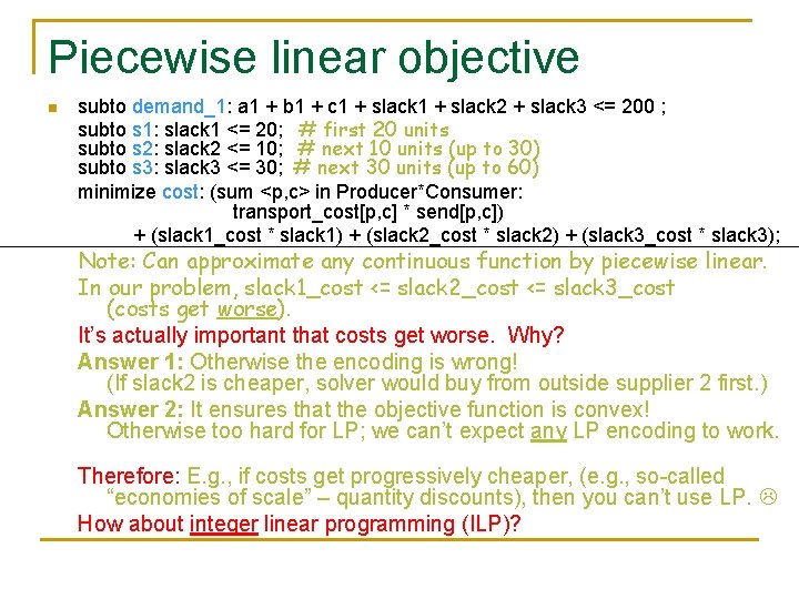
Piecewise linear objective n subto demand_1: a 1 + b 1 + c 1 + slack 2 + slack 3 <= 200 ; subto s 1: slack 1 <= 20; # first 20 units subto s 2: slack 2 <= 10; # next 10 units (up to 30) subto s 3: slack 3 <= 30; # next 30 units (up to 60) minimize cost: (sum <p, c> in Producer*Consumer: transport_cost[p, c] * send[p, c]) + (slack 1_cost * slack 1) + (slack 2_cost * slack 2) + (slack 3_cost * slack 3); Note: Can approximate any continuous function by piecewise linear. In our problem, slack 1_cost <= slack 2_cost <= slack 3_cost (costs get worse). It’s actually important that costs get worse. Why? Answer 1: Otherwise the encoding is wrong! (If slack 2 is cheaper, solver would buy from outside supplier 2 first. ) Answer 2: It ensures that the objective function is convex! Otherwise too hard for LP; we can’t expect any LP encoding to work. Therefore: E. g. , if costs get progressively cheaper, (e. g. , so-called “economies of scale” – quantity discounts), then you can’t use LP. How about integer linear programming (ILP)?

Piecewise linear objective n subto demand_1: a 1 + b 1 + c 1 + slack 2 + slack 3 <= 200 ; subto s 1: slack 1 <= 20; # first 20 units subto s 2: slack 2 <= 10; # next 10 units (up to 30) subto s 3: slack 3 <= 30; # next 30 units (up to 60) minimize cost: (sum <p, c> in Producer*Consumer: transport_cost[p, c] * send[p, c]) + (slack 1_cost * slack 1) + (slack 2_cost * slack 2) + (slack 3_cost * slack 3); n Need to ensure that even if the slack_costs are set arbitrarily (any function!), slack 1 must reach 20 before we can get the quantity discount by using slack 2. Use integer linear programming. How? var k 1 binary; var k 2 binary; var k 3 binary; # 0 -1 ILP subto slack 1 <= 20*k 1; # can only use slack 1 if k 1==1, not if k 1==0 If we want to allow total slack, should we drop this constraint? subto slack 2 <= 10*k 2; No, we need it (if k 3==0). Just change 30 to a large number M. subto slack 3 <= 30*k 3; (If slack 3 reaches M in the solution, increase M and try again. ) subto slack 1 >= k 2*20; # if we use slack 2, then slack 1 must be fully used subto slack 2 >= k 3*10; # if we use slack 3, then slack 2 must be fully used n n Can drop k 1. It really has no effect, since nothing stops it from being 1. Corresponds to the fact that we’re always allowed to use slack 1.

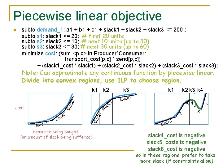
Piecewise linear objective n subto demand_1: a 1 + b 1 + c 1 + slack 2 + slack 3 <= 200 ; subto s 1: slack 1 <= 20; # first 20 units subto s 2: slack 2 <= 10; # next 10 units (up to 30) subto s 3: slack 3 <= 30; # next 30 units (up to 60) minimize cost: (sum <p, c> in Producer*Consumer: transport_cost[p, c] * send[p, c]) + (slack 1_cost * slack 1) + (slack 2_cost * slack 2) + (slack 3_cost * slack 3); Note: Can approximate any continuous function by piecewise linear. Divide into convex regions, use ILP to choose region. 2 k 3 k 4 slack 3 34 sla ck a l s slack 1 resource being bought (or amount of slack being suffered) 2 ck 1 k 2 c sla k 1 5 cost k 3 7 ck 3 k 1 k 2 6 k 1 slack 4_cost is negative slack 5_costs is negative slack 6_cost is negative so in these regions, prefer to take more slack (if constraints allow)

Image Alignment 600. 325/425 Declarative Methods - J. Eisner 48

Image Alignment as a transportation problem, via “Earth Mover’s Distance” (Monge, 1781) 600. 325/425 Declarative Methods - J. Eisner 49

Image Alignment as a transportation problem, via “Earth Mover’s Distance” (Monge, 1781) 600. 325/425 Declarative Methods - J. Eisner 50

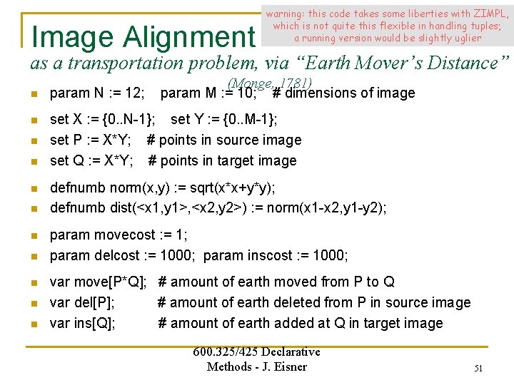
Image Alignment warning: this code takes some liberties with ZIMPL, which is not quite this flexible in handling tuples; a running version would be slightly uglier as a transportation problem, via “Earth Mover’s Distance” (Monge, 1781) param M : = 10; # dimensions of image n param N : = 12; n set X : = {0. . N-1}; set Y : = {0. . M-1}; set P : = X*Y; # points in source image set Q : = X*Y; # points in target image n n n n n defnumb norm(x, y) : = sqrt(x*x+y*y); defnumb dist(<x 1, y 1>, <x 2, y 2>) : = norm(x 1 -x 2, y 1 -y 2); param movecost : = 1; param delcost : = 1000; param inscost : = 1000; var move[P*Q]; # amount of earth moved from P to Q var del[P]; # amount of earth deleted from P in source image var ins[Q]; # amount of earth added at Q in target image 600. 325/425 Declarative Methods - J. Eisner 51

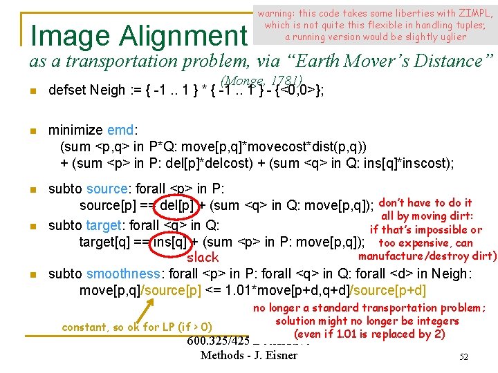
Image Alignment warning: this code takes some liberties with ZIMPL, which is not quite this flexible in handling tuples; a running version would be slightly uglier as a transportation problem, via “Earth Mover’s Distance” n (Monge, 1781) defset Neigh : = { -1. . 1 } * { -1. . 1 } - {<0, 0>}; n minimize emd: (sum <p, q> in P*Q: move[p, q]*movecost*dist(p, q)) + (sum <p> in P: del[p]*delcost) + (sum <q> in Q: ins[q]*inscost); n subto source: forall <p> in P: source[p] == del[p] + (sum <q> in Q: move[p, q]); don’t have to do it all by moving dirt: subto target: forall <q> in Q: if that’s impossible or target[q] == ins[q] + (sum <p> in P: move[p, q]); too expensive, can manufacture/destroy dirt) slack subto smoothness: forall <p> in P: forall <q> in Q: forall <d> in Neigh: move[p, q]/source[p] <= 1. 01*move[p+d, q+d]/source[p+d] n n constant, so ok for LP (if > 0) no longer a standard transportation problem; solution might no longer be integers (even if 1. 01 is replaced by 2) 600. 325/425 Declarative Methods - J. Eisner 52

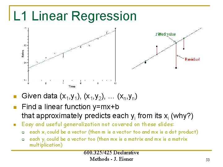
L 1 Linear Regression n Given data (x 1, y 1), (x 1, y 2), … (xn, yn) Find a linear function y=mx+b that approximately predicts each yi from its xi (why? ) Easy and useful generalization not covered on these slides: q q each xi could be a vector (then m is a vector too and mx is a dot product) each yi could be a vector too (then mx is a matrix and mx is a matrix multiplication) 600. 325/425 Declarative Methods - J. Eisner 53

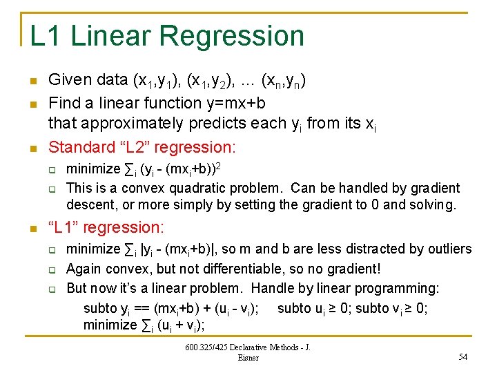
L 1 Linear Regression n Given data (x 1, y 1), (x 1, y 2), … (xn, yn) Find a linear function y=mx+b that approximately predicts each yi from its xi Standard “L 2” regression: q q n minimize ∑i (yi - (mxi+b))2 This is a convex quadratic problem. Can be handled by gradient descent, or more simply by setting the gradient to 0 and solving. “L 1” regression: q q q minimize ∑i |yi - (mxi+b)|, so m and b are less distracted by outliers Again convex, but not differentiable, so no gradient! But now it’s a linear problem. Handle by linear programming: subto yi == (mxi+b) + (ui - vi); subto ui ≥ 0; subto vi ≥ 0; minimize ∑i (ui + vi); 600. 325/425 Declarative Methods - J. Eisner 54

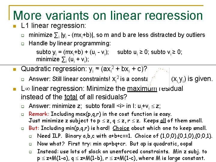
More variants on linear regression n L 1 linear regression: q q n n minimize ∑i |yi - (mxi+b)|, so m and b are less distracted by outliers Handle by linear programming: subto yi = (mxi+b) + (ui - vi); subto ui ≥ 0; subto vi ≥ 0; you’ve heard of Ridge or Lasso regression: “Regularize” m (encourage minimize ∑i (ui + vi); If it to be small) by adding ||m|| to objective function, under L 2 or L 1 norm Quadratic regression: yi ≈ (axi 2 + bxi + c)? 2 q Answer: Still linear constraints! xi is a constant since (xi, yi) is given. L linear regression: Minimize the maximum residual instead of the total of all residuals? q q q Answer: minimize z; subto forall <i> in I: ui+vi z; Remark: Including max(p, q, r) in the cost function is easy. Just minimize z subject to p z, q z, r z. Keeps all of them small. But: Including min(p, q, r) is hard! Choice about which one to keep small. q Need ILP. Binary a, b, c with a+b+c==1. Choice of (1, 0, 0), (0, 1, 0), (0, 0, 1). q Now what? First try: min ap+bq+cr. But ap is quadratic, oops! Methods - J. constraints. Min z subj. to q Instead: use lots 600. 325/425 of slack. Declarative on unenforced 55 Eisner p z+M(1 -a), q z+M(1 -b), r z+M(1 -c), where M is large constant.

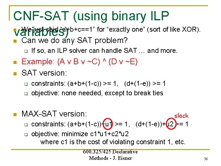
CNF-SAT (using binary ILP We just said “a+b+c==1” for “exactly one” (sort of like XOR). variables) n n Can we do any SAT problem? q n n Example: (A v B v ~C) ^ (D v ~E) SAT version: q q n If so, an ILP solver can handle SAT … and more. constraints: (a+b+(1 -c)) >= 1, (d+(1 -e)) >= 1 objective: none needed, except to break ties MAX-SAT version: q q slack constraints: (a+b+(1 -c))+u 1 >= 1, (d+(1 -e))+u 2 >= 1 objective: minimize c 1*u 1+c 2*u 2 where c 1 is the cost of violating constraint 1, etc. 600. 325/425 Declarative Methods - J. Eisner 56

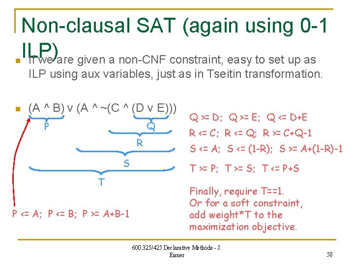
n n Non-clausal SAT (again using 0 -1 ILP) If A is a [boolean] variable, then A and ~A are “literal” formulas. If F and G are formulas, then so are q q q n F ^ G (“F and G”) F v G (“F or G”) F G (“If F then G”; “F implies G”) F G (“F if and only if G”; “F is equivalent to G”) F xor G (“F or G but not both”; “F differs from G”) ~F (“not F”) If we are given a non-clausal formula, easy to set up as ILP. q q Use aux variables exactly as in Tseitin transformation. Need only a linear number of new variables and new constraints. 600. 325/425 Declarative Methods - J. Eisner 57

n Non-clausal SAT (again using 0 -1 ILP) If we are given a non-CNF constraint, easy to set up as ILP using aux variables, just as in Tseitin transformation. n (A ^ B) v (A ^ ~(C ^ (D v E))) Q P R S T P <= A; P <= B; P >= A+B-1 Q >= D; Q >= E; Q <= D+E R <= C; R <= Q; R >= C+Q-1 S <= A; S <= (1 -R); S >= A+(1 -R)-1 T >= P; T >= S; T <= P+S Finally, require T==1. Or for a soft constraint, add weight*T to the maximization objective. 600. 325/425 Declarative Methods - J. Eisner 58

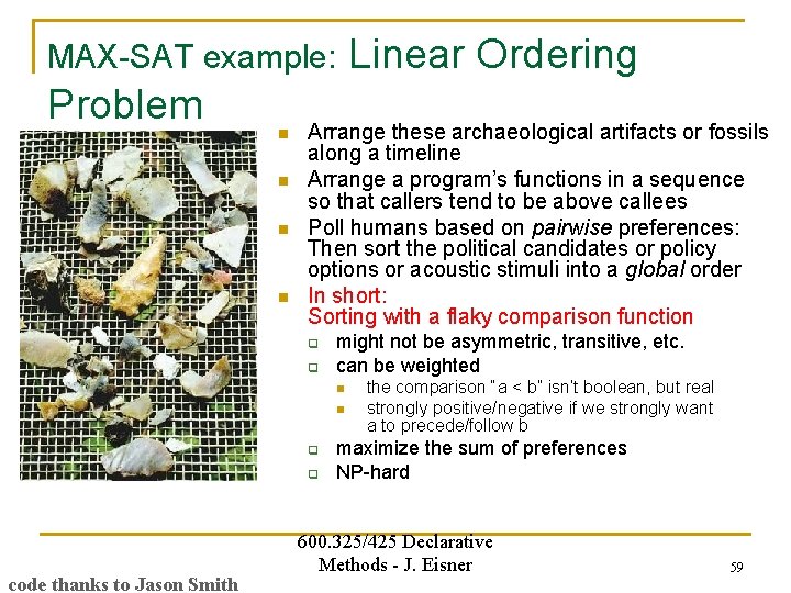
MAX-SAT example: Problem n n Arrange these archaeological artifacts or fossils along a timeline Arrange a program’s functions in a sequence so that callers tend to be above callees Poll humans based on pairwise preferences: Then sort the political candidates or policy options or acoustic stimuli into a global order In short: Sorting with a flaky comparison function q q might not be asymmetric, transitive, etc. can be weighted n n q q code thanks to Jason Smith Linear Ordering the comparison “a < b” isn’t boolean, but real strongly positive/negative if we strongly want a to precede/follow b maximize the sum of preferences NP-hard 600. 325/425 Declarative Methods - J. Eisner 59

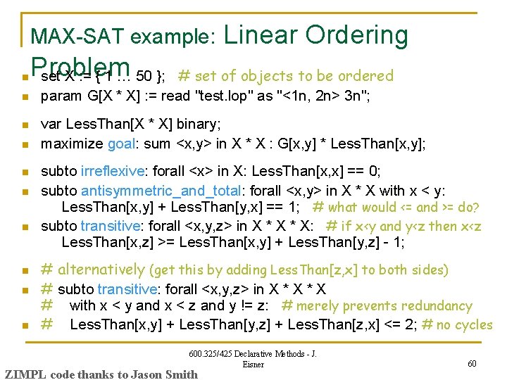
MAX-SAT example: n n n n n Linear Ordering Problem set X : = { 1 … 50 }; # set of objects to be ordered param G[X * X] : = read "test. lop" as "<1 n, 2 n> 3 n"; var Less. Than[X * X] binary; maximize goal: sum <x, y> in X * X : G[x, y] * Less. Than[x, y]; subto irreflexive: forall <x> in X: Less. Than[x, x] == 0; subto antisymmetric_and_total: forall <x, y> in X * X with x < y: Less. Than[x, y] + Less. Than[y, x] == 1; # what would <= and >= do? subto transitive: forall <x, y, z> in X * X: # if x<y and y<z then x<z Less. Than[x, z] >= Less. Than[x, y] + Less. Than[y, z] - 1; # alternatively (get this by adding Less. Than[z, x] to both sides) # subto transitive: forall <x, y, z> in X * X # with x < y and x < z and y != z: # merely prevents redundancy # Less. Than[x, y] + Less. Than[y, z] + Less. Than[z, x] <= 2; # no cycles 600. 325/425 Declarative Methods - J. Eisner ZIMPL code thanks to Jason Smith 60

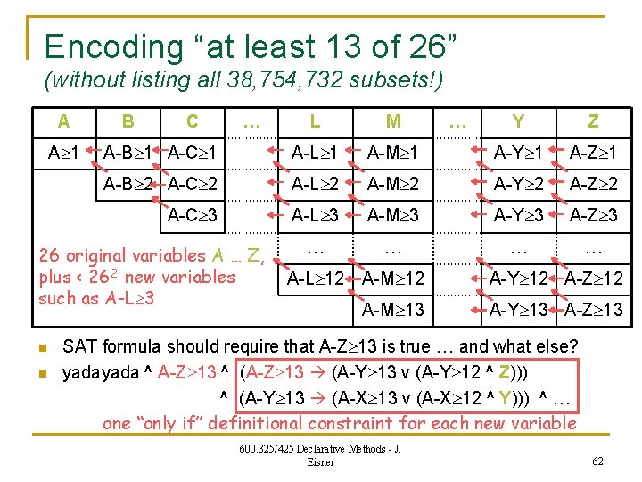
Why isn’t this just SAT all over again? n n Different solution techniques (we’ll compare) Much easier to encode “at least 13 of 26”: q Remember how we had to do it in pure SAT?

Encoding “at least 13 of 26” (without listing all 38, 754, 732 subsets!) A A 1 B C … L M A-B 1 A-C 1 A-L 1 A-B 2 A-C 3 26 original variables A … Z, plus < 262 new variables such as A-L 3 n n … Y Z A-M 1 A-Y 1 A-Z 1 A-L 2 A-M 2 A-Y 2 A-Z 2 A-L 3 A-M 3 A-Y 3 A-Z 3 … … A-L 12 A-M 12 A-Y 12 A-Z 12 A-M 13 A-Y 13 A-Z 13 SAT formula should require that A-Z 13 is true … and what else? yada ^ A-Z 13 ^ (A-Z 13 (A-Y 13 v (A-Y 12 ^ Z))) ^ (A-Y 13 (A-X 13 v (A-X 12 ^ Y))) ^ … one “only if” definitional constraint for each new variable 600. 325/425 Declarative Methods - J. Eisner 62

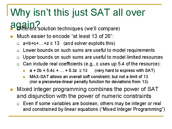
Why isn’t this just SAT all over again? Different solution techniques (we’ll compare) n n Much easier to encode “at least 13 of 26”: q q a+b+c+…+z ≥ 13 (and solver exploits this) Lower bounds on such sums are useful to model requirements Upper bounds on such sums are useful to model limited resources Can include real coefficients (e. g. , c uses up 5. 4 of the resource): n n n a + 2 b + 5. 4 c + … + 0. 3 z ≥ 13 (very hard to express with SAT) MAX-SAT allows an overall soft constraint, but not a limit of 13 (nor a piecewise-linear penalty function for deviations from 13) Mixed integer programming combines the power of SAT and disjunction with the power of numeric constraints q Even if some variables are boolean, others may be integer or real and constrained by linear equations (“Mixed Integer Programming”)

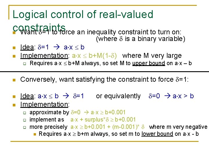
Logical control of real-valued constraints n Want =1 to force an inequality constraint to turn on: (where is a binary variable) n n Idea: =1 a x b Implementation: a x b+M(1 - ) where M very large q n n n Requires a x b+M always, so set M to upper bound on a x – b Conversely, want satisfying the constraint to force =1: Idea: a x b =1 Implementation: q q q or equivalently =0 a x > b approximate by =0 a x b+0. 001 implement as a x + surplus* b+0. 001 more precisely a x b+0. 001 + (m-0. 001)* where m very negative n Requires a x b+m always, so set m to lower bound on a x - b

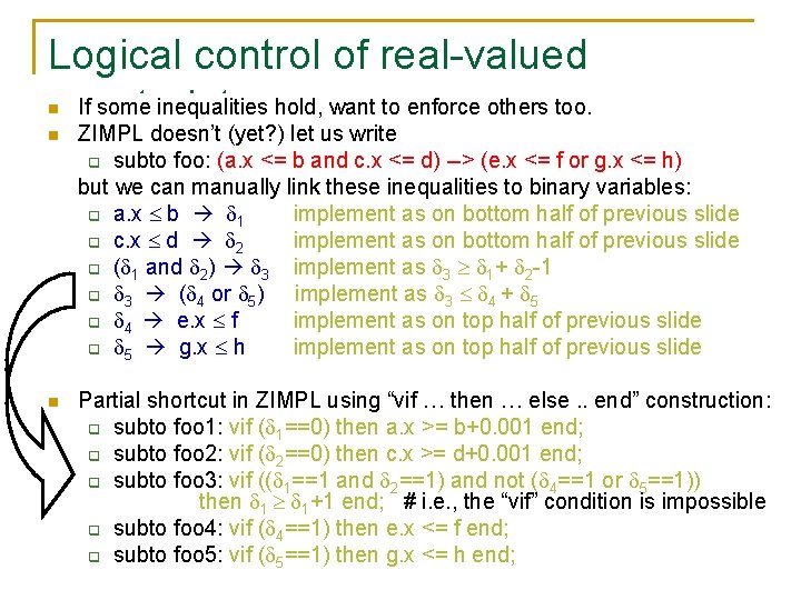
Logical control of real-valued If some inequalities hold, want to enforce others too. constraints n n ZIMPL doesn’t (yet? ) let us write q subto foo: (a. x <= b and c. x <= d) --> (e. x <= f or g. x <= h) but we can manually link these inequalities to binary variables: q a. x b 1 implement as on bottom half of previous slide q c. x d 2 implement as on bottom half of previous slide q ( 1 and 2) 3 implement as 3 1+ 2 -1 q 3 ( 4 or 5) implement as 3 4 + 5 q 4 e. x f implement as on top half of previous slide q 5 g. x h implement as on top half of previous slide n Partial shortcut in ZIMPL using “vif … then … else. . end” construction: q subto foo 1: vif ( 1==0) then a. x >= b+0. 001 end; q subto foo 2: vif ( 2==0) then c. x >= d+0. 001 end; q subto foo 3: vif (( 1==1 and 2==1) and not ( 4==1 or 5==1)) then 1 1+1 end; # i. e. , the “vif” condition is impossible q subto foo 4: vif ( 4==1) then e. x <= f end; q subto foo 5: vif ( 5==1) then g. x <= h end;

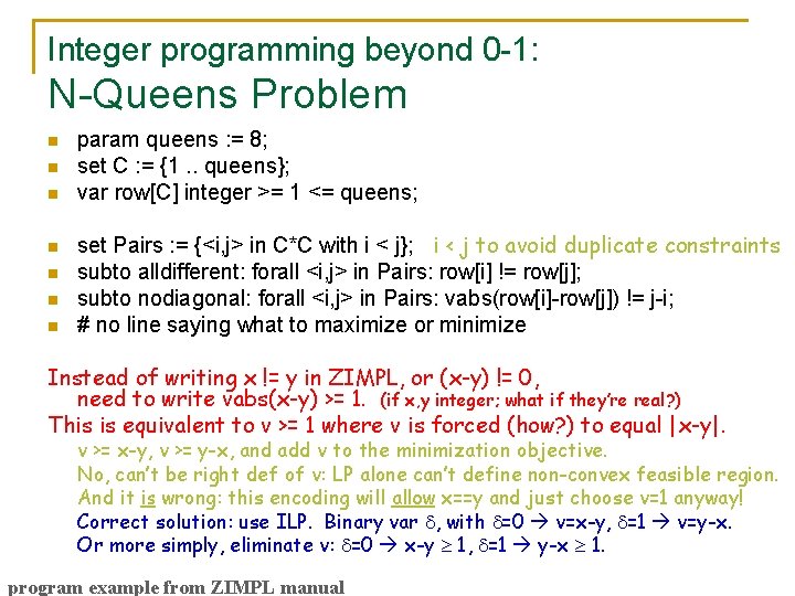
Integer programming beyond 0 -1: N-Queens Problem n n n n param queens : = 8; set C : = {1. . queens}; var row[C] integer >= 1 <= queens; set Pairs : = {<i, j> in C*C with i < j}; i < j to avoid duplicate constraints subto alldifferent: forall <i, j> in Pairs: row[i] != row[j]; subto nodiagonal: forall <i, j> in Pairs: vabs(row[i]-row[j]) != j-i; # no line saying what to maximize or minimize Instead of writing x != y in ZIMPL, or (x-y) != 0, need to write vabs(x-y) >= 1. (if x, y integer; what if they’re real? ) This is equivalent to v >= 1 where v is forced (how? ) to equal |x-y|. v >= x-y, v >= y-x, and add v to the minimization objective. No, can’t be right def of v: LP alone can’t define non-convex feasible region. And it is wrong: this encoding will allow x==y and just choose v=1 anyway! Correct solution: use ILP. Binary var , with =0 v=x-y, =1 v=y-x. Or more simply, eliminate v: =0 x-y 1, =1 y-x 1. program example from ZIMPL manual

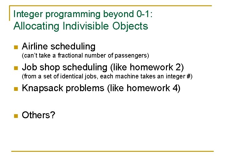
Integer programming beyond 0 -1: Allocating Indivisible Objects n Airline scheduling (can’t take a fractional number of passengers) n Job shop scheduling (like homework 2) (from a set of identical jobs, each machine takes an integer #) n Knapsack problems (like homework 4) n Others?

Harder Real-World Examples of LP/ILP/MIP

Unsupervised Learning of a Part-of-Speech Tagger n based on Ravi & Knight 2009 600. 325/425 Declarative Methods - J. Eisner 69

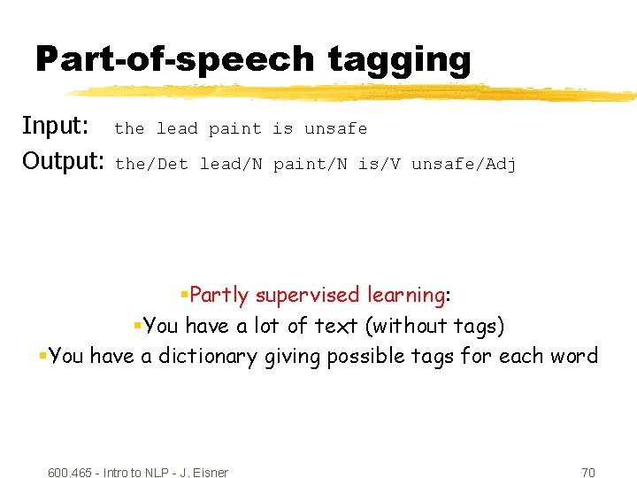
Part-of-speech tagging Input: the lead paint Output: the/Det lead/N is unsafe paint/N is/V unsafe/Adj §Partly supervised learning: §You have a lot of text (without tags) §You have a dictionary giving possible tags for each word 600. 465 - Intro to NLP - J. Eisner 70

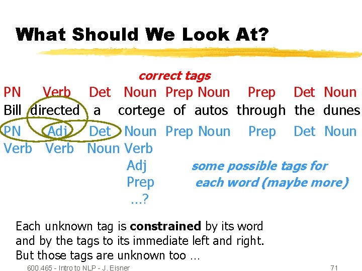
What Should We Look At? correct tags PN Verb Bill directed PN Adj Verb Det Noun Prep Det Noun a cortege of autos through the dunes Det Noun Prep Det Noun Verb Adj some possible tags for Prep each word (maybe more) …? Each unknown tag is constrained by its word and by the tags to its immediate left and right. But those tags are unknown too … 600. 465 - Intro to NLP - J. Eisner 71

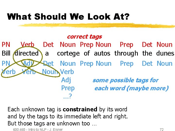
What Should We Look At? correct tags PN Verb Bill directed PN Adj Verb Det Noun Prep Det Noun a cortege of autos through the dunes Det Noun Prep Det Noun Verb Adj some possible tags for Prep each word (maybe more) …? Each unknown tag is constrained by its word and by the tags to its immediate left and right. But those tags are unknown too … 600. 465 - Intro to NLP - J. Eisner 72

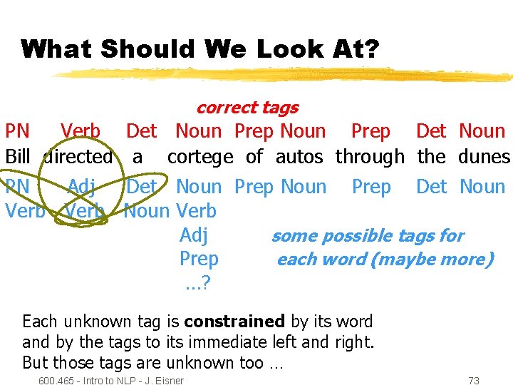
What Should We Look At? correct tags PN Verb Bill directed PN Adj Verb Det Noun Prep Det Noun a cortege of autos through the dunes Det Noun Prep Det Noun Verb Adj some possible tags for Prep each word (maybe more) …? Each unknown tag is constrained by its word and by the tags to its immediate left and right. But those tags are unknown too … 600. 465 - Intro to NLP - J. Eisner 73

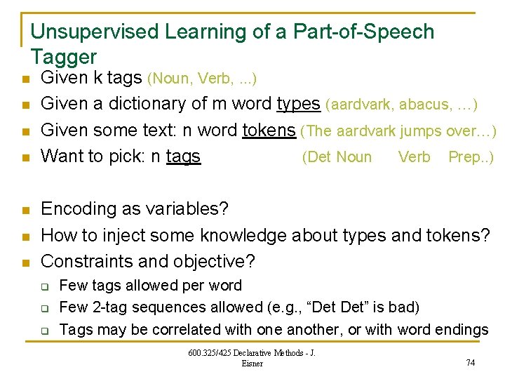
Unsupervised Learning of a Part-of-Speech Tagger n n n n Given k tags (Noun, Verb, . . . ) Given a dictionary of m word types (aardvark, abacus, …) Given some text: n word tokens (The aardvark jumps over…) Want to pick: n tags (Det Noun Verb Prep. . ) Encoding as variables? How to inject some knowledge about types and tokens? Constraints and objective? q q q Few tags allowed per word Few 2 -tag sequences allowed (e. g. , “Det Det” is bad) Tags may be correlated with one another, or with word endings 600. 325/425 Declarative Methods - J. Eisner 74

Minimum spanning tree ++ n based on Martins et al. 2009 600. 325/425 Declarative Methods - J. Eisner 75

Traveling Salesperson n Version with subtour elimination constraints n Version with auxiliary variables