Chapter 9 Function Approximation 2003010594 2004020594 2005020594 Korea

Chapter 9 Function Approximation 고려대학교 컴퓨터학과 음성정보처리 연구실 2003010594 조영규 2004020594 방규섭 2005020594 정재연

Korea Universit y Contents 9. 1 Least Squares Approximation 9. 2 Continuous Least Squares 9. 3 Function Approximation at a Point 9. 4 Using Matlab’s Functions 음성정보처리연구실 2

9. 1 Least Squares Approximation Korea Universit y Some of the most common methods of approximating data are based on the desire to minimize some measure of the difference between the approximating function and the given data points. The method of least squares seeks to minimize the sum of the squares of the differences between the function value and the data value. Advantages to using the square of the differences at each point Positive differences do not cancel negative differences Differentiation is not difficult Small differences become smaller and large differences are magnified 음성정보처리연구실 3

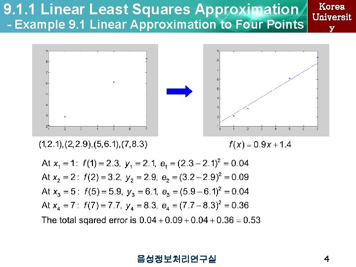
9. 1. 1 Linear Least Squares Approximation - Example 9. 1 Linear Approximation to Four Points 음성정보처리연구실 Korea Universit y 4

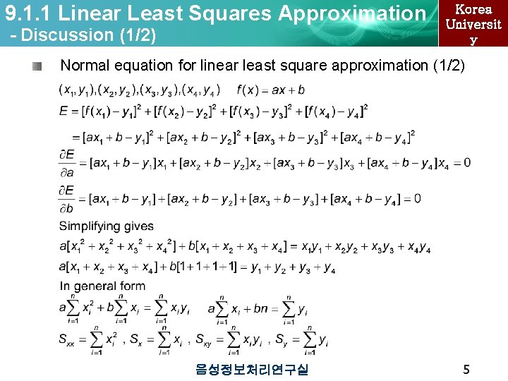
9. 1. 1 Linear Least Squares Approximation - Discussion (1/2) Korea Universit y Normal equation for linear least square approximation (1/2) 음성정보처리연구실 5

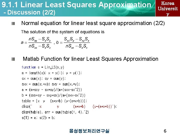
9. 1. 1 Linear Least Squares Approximation - Discussion (2/2) Korea Universit y Normal equation for linear least square approximation (2/2) Matlab Function for linear Least Squares Approximation 음성정보처리연구실 6

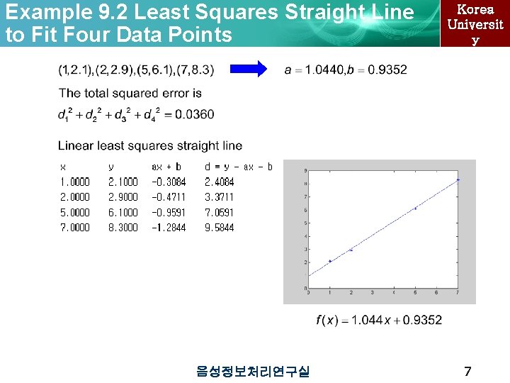
Example 9. 2 Least Squares Straight Line to Fit Four Data Points 음성정보처리연구실 Korea Universit y 7

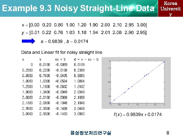
Example 9. 3 Noisy Straight-Line Data 음성정보처리연구실 Korea Universit y 8

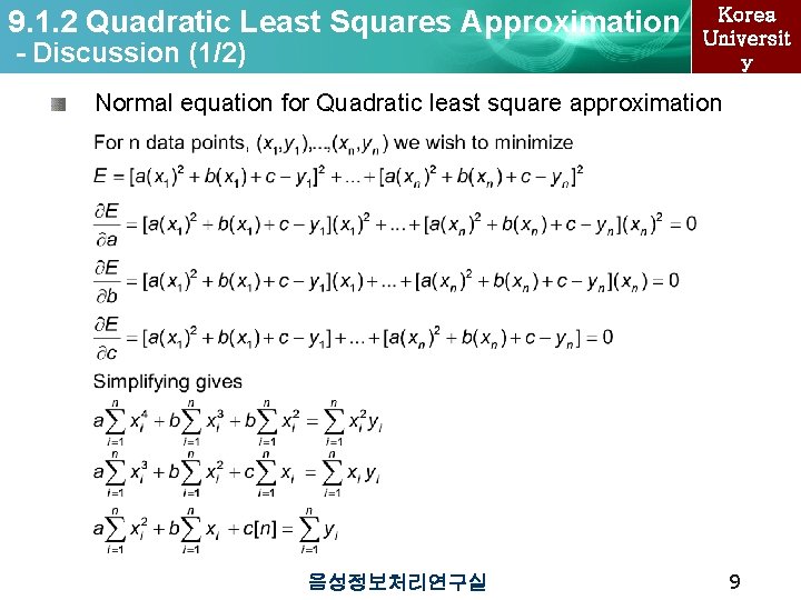
9. 1. 2 Quadratic Least Squares Approximation - Discussion (1/2) Korea Universit y Normal equation for Quadratic least square approximation 음성정보처리연구실 9

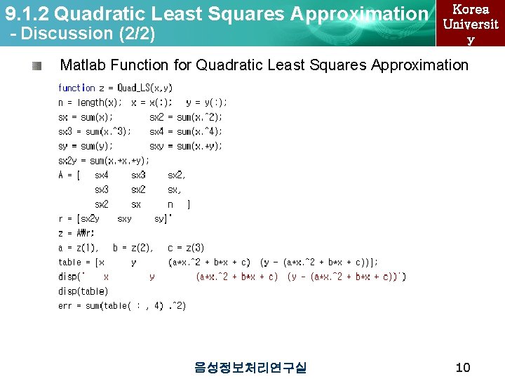
9. 1. 2 Quadratic Least Squares Approximation - Discussion (2/2) Korea Universit y Matlab Function for Quadratic Least Squares Approximation 음성정보처리연구실 10

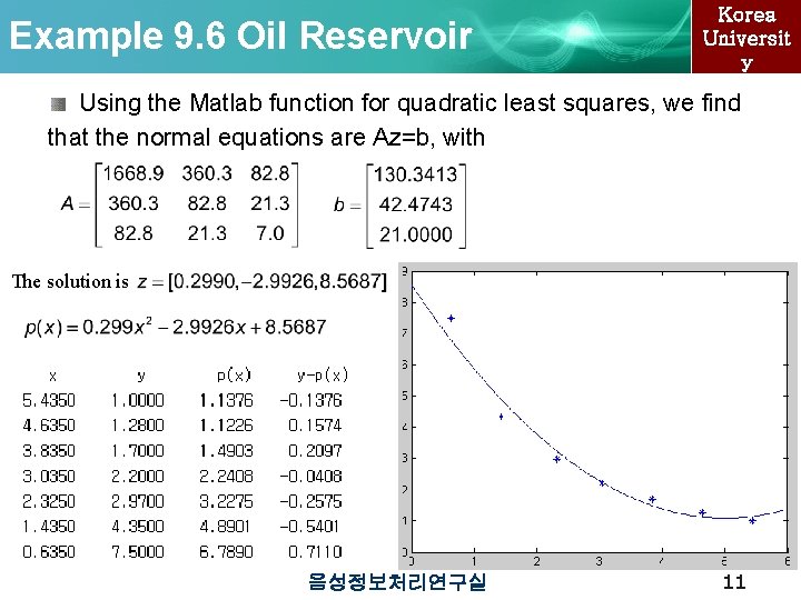
Example 9. 6 Oil Reservoir Korea Universit y Using the Matlab function for quadratic least squares, we find that the normal equations are Az=b, with The solution is 음성정보처리연구실 11

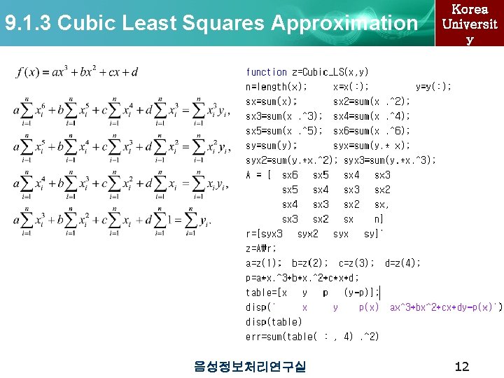
9. 1. 3 Cubic Least Squares Approximation 음성정보처리연구실 Korea Universit y 12

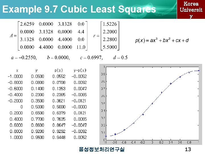
Example 9. 7 Cubic Least Squares 음성정보처리연구실 Korea Universit y 13

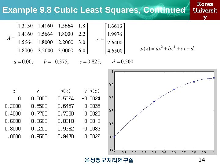
Example 9. 8 Cubic Least Squares, Continued 음성정보처리연구실 Korea Universit y 14

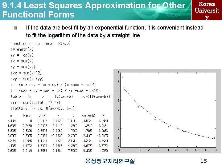
9. 1. 4 Least Squares Approximation for Other Functional Forms Korea Universit y If the data are best fit by an exponential function, it is convenient instead to fit the logarithm of the data by a straight line 음성정보처리연구실 15

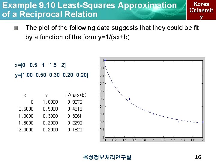
Example 9. 10 Least-Squares Approximation of a Reciprocal Relation Korea Universit y The plot of the following data suggests that they could be fit by a function of the form y=1/(ax+b) x=[0 0. 5 1 1. 5 2] y=[1. 00 0. 50 0. 30 0. 20] 음성정보처리연구실 16

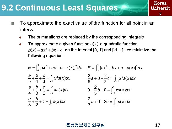
9. 2 Continuous Least Squares Korea Universit y To approximate the exact value of the function for all point in an interval The summations are replaced by the corresponding integrals To approximate a given function a quadratic function on the interval [0, 1] and [-1, 1], we minimize the following equation. 음성정보처리연구실 17

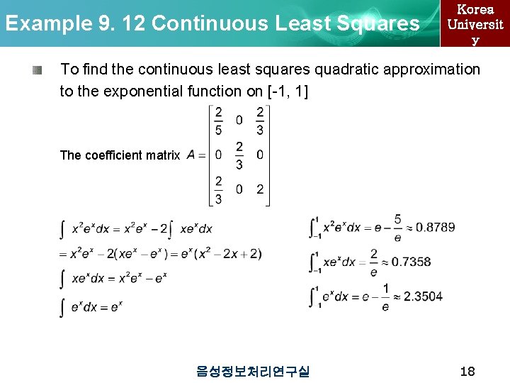
Example 9. 12 Continuous Least Squares Korea Universit y To find the continuous least squares quadratic approximation to the exponential function on [-1, 1] The coefficient matrix 음성정보처리연구실 18

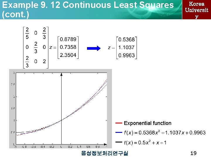
Example 9. 12 Continuous Least Squares (cont. ) Korea Universit y Exponential function 음성정보처리연구실 19

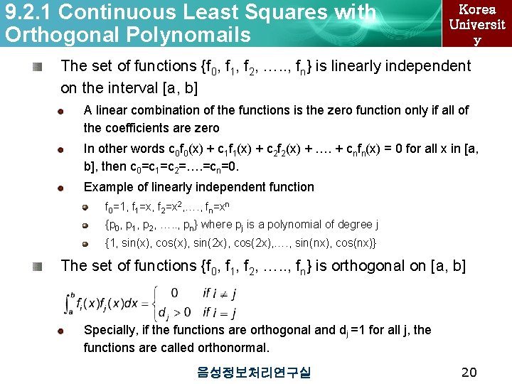
9. 2. 1 Continuous Least Squares with Orthogonal Polynomails Korea Universit y The set of functions {f 0, f 1, f 2, …. . , fn} is linearly independent on the interval [a, b] A linear combination of the functions is the zero function only if all of the coefficients are zero In other words c 0 f 0(x) + c 1 f 1(x) + c 2 f 2(x) + …. + cnfn(x) = 0 for all x in [a, b], then c 0=c 1=c 2=…. =cn=0. Example of linearly independent function f 0=1, f 1=x, f 2=x 2, …. , fn=xn {p 0, p 1, p 2, …. . , pn} where pj is a polynomial of degree j {1, sin(x), cos(x), sin(2 x), cos(2 x), …. , sin(nx), cos(nx)} The set of functions {f 0, f 1, f 2, …. . , fn} is orthogonal on [a, b] Specially, if the functions are orthogonal and dj =1 for all j, the functions are called orthonormal. 음성정보처리연구실 20

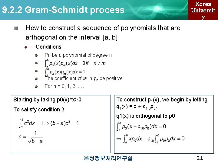
9. 2. 2 Gram-Schmidt process Korea Universit y How to construct a sequence of polynomials that are arthogonal on the interval [a, b] Conditions Pn be a polynomial of degree n The coefficient of xn in pn be positive For n = 0, 1, 2, …. Starting by taking p 0(x)=x>0 To satisfy condition 3 To construct p 1(x), we begin by letting q 1(x) = x + c 1, 0 p 0. q 1(x) is orthogonal to p 0 음성정보처리연구실 21

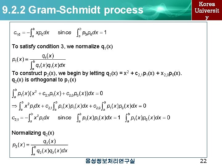
9. 2. 2 Gram-Schmidt process Korea Universit y To satisfy condition 3, we normalize q 1(x) To construct p 2(x), we begin by letting q 2(x) = x 2 + c 2, 1 p 1(x) + x 2, 0 p 0(x). q 2(x) is orthogonal to p 1(x) Normalizing q 2(x) 음성정보처리연구실 22

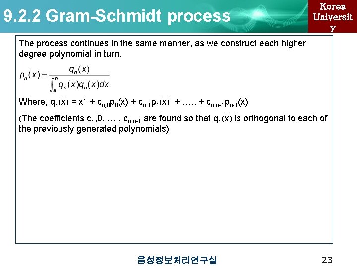
9. 2. 2 Gram-Schmidt process Korea Universit y The process continues in the same manner, as we construct each higher degree polynomial in turn. Where, qn(x) = xn + cn, 0 p 0(x) + cn, 1 p 1(x) + …. . + cn, n-1 pn-1(x) (The coefficients cn, 0, … , cn, n-1 are found so that qn(x) is orthogonal to each of the previously generated polynomials) 음성정보처리연구실 23

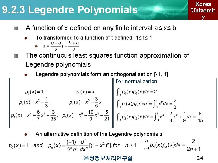
9. 2. 3 Legendre Polynomials Korea Universit y A function of x defined on any finite interval a≤ x≤ b To transformed to a function of t defined -1≤ t≤ 1 The continuous least squares function approximation of Legendre polynomials form an orthogonal set on [-1, 1] For normalization An alternative definition of the Legendre polynomials 음성정보처리연구실 24

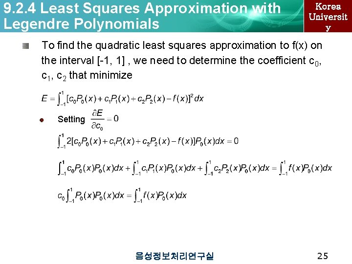
9. 2. 4 Least Squares Approximation with Legendre Polynomials Korea Universit y To find the quadratic least squares approximation to f(x) on the interval [-1, 1] , we need to determine the coefficient c 0, c 1, c 2 that minimize Setting 음성정보처리연구실 25

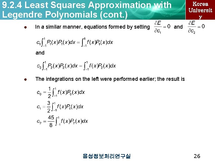
9. 2. 4 Least Squares Approximation with Legendre Polynomials (cont. ) In a similar manner, equations formed by setting Korea Universit y and The integrations on the left were performed earlier; the result is 음성정보처리연구실 26

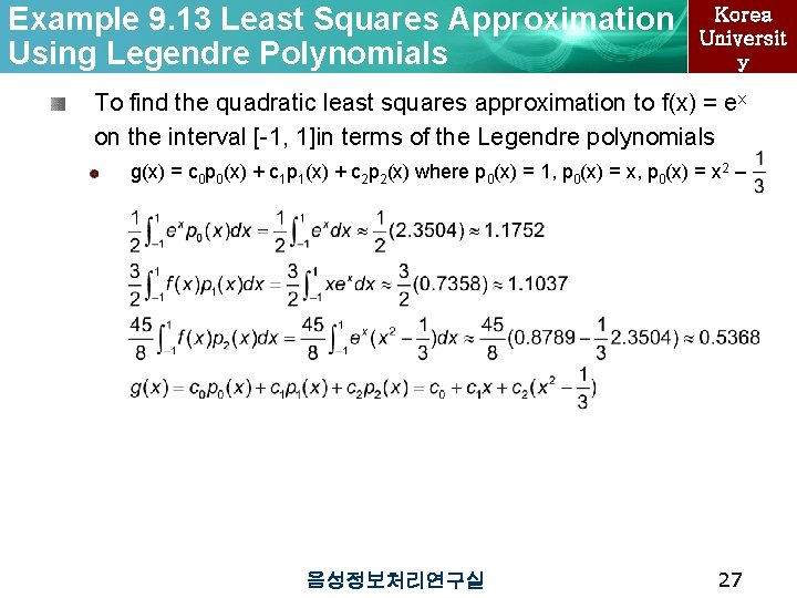
Example 9. 13 Least Squares Approximation Using Legendre Polynomials Korea Universit y To find the quadratic least squares approximation to f(x) = ex on the interval [-1, 1]in terms of the Legendre polynomials g(x) = c 0 p 0(x) + c 1 p 1(x) + c 2 p 2(x) where p 0(x) = 1, p 0(x) = x 2 – 음성정보처리연구실 27

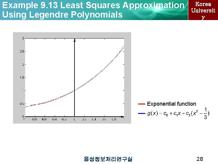
Example 9. 13 Least Squares Approximation Using Legendre Polynomials Korea Universit y Exponential function 음성정보처리연구실 28

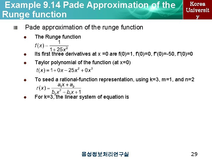
Example 9. 14 Pade Approximation of the Runge function Korea Universit y Pade approximation of the runge function The Runge function Its first three derivatives at x =0 are f(0)=1, f′(0)=0, f″(0)=-50, f‴(0)=0 Taylor polynomial of the function (at x=0) To seed a rational-function representation, using k=3, m=1, and n=2 For k=3, the linear system of equation is 음성정보처리연구실 29

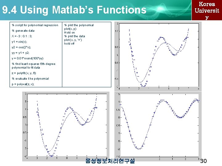
9. 4 Using Matlab’s Functions % script for polynomial regression % generate data X = -3 : 0. 1 : 3; y 1 = sin(x); Korea Universit y % plot the polynomial plot(x, p) Hold on % plot the data plot (x, y, ‘+’) hold off y 2 = cos(2*x); yy = y 1 + y 2; y = 0. 01*round(100*yy) % find least squares 6 th-degree polynomial to fit data z = polyfit (x, y, 6) % evaluate t he polynomial p = polyval(z, x); 음성정보처리연구실 30