Approximation Algorithms Spring 2007 Approximation Algorithms 1 Outline

Approximation Algorithms Spring 2007 Approximation Algorithms 1

Outline and Reading Approximation Algorithms for NP-Complete Problems (§ 13. 4) n n n Approximation ratios Polynomial-Time Approximation Schemes (§ 13. 4. 1) PTAS for 0/1 Knapsack 2 -Approximation for Vertex Cover (§ 13. 4. 2) 2 -Approximation for TSP special case (§ 13. 4. 3) Log n-Approximation for Set Cover (§ 13. 4. 4) Spring 2007 Approximation Algorithms 2

Approximation Ratios Optimization Problems n n We have some problem instance x that has many feasible “solutions”. We are trying to minimize (or maximize) some cost function c(S) for a “solution” S to x. For example, w Finding a minimum spanning tree of a graph w Finding a smallest vertex cover of a graph w Finding a smallest traveling salesperson tour in a graph Spring 2007 Approximation Algorithms 3

Approximation Ratios An approximation produces a solution T is a δ-approximation to the optimal solution if c(T) ≤ δ OPT (assuming a minimization problem). w OPT ≤ δ c(T) for a maximization problem w In both cases we assume δ>1 Spring 2007 Approximation Algorithms 4

Polynomial-Time Approximation Schemes A problem L has a polynomial-time approximation scheme (PTAS) if for any fixed >0 it has a (1+ )-approximation algorithm that runs in polynomial time n Polynomial time based on input size n, though may also appear in the expression for run time. A problem has a fully polynomial-time approximation scheme (FPTAS) if the run time is polynomial in both n and 1/ 0/1 Knapsack has a FPTAS, with a running time that is O(n 3/ ). Spring 2007 Approximation Algorithms 5

PTAS for 0/1 Knapsack Problem: Set S of items numbered 1, …, n. n Constraint (total size limit) s n Item i has size si and worth wi n Want to find subset T that maximizes the worth Spring 2007 Approximation Algorithms 6

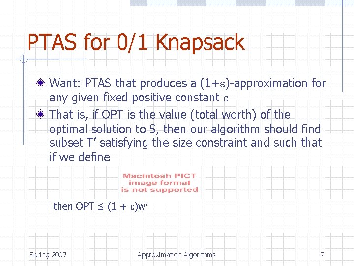
PTAS for 0/1 Knapsack Want: PTAS that produces a (1+ )-approximation for any given fixed positive constant That is, if OPT is the value (total worth) of the optimal solution to S, then our algorithm should find subset T’ satisfying the size constraint and such that if we define then OPT ≤ (1 + )w Spring 2007 Approximation Algorithms 7

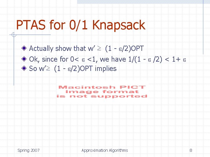
PTAS for 0/1 Knapsack Actually show that w’ ≥ (1 - /2)OPT Ok, since for 0< <1, we have 1/(1 - /2) < 1+ So w’≥ (1 - /2)OPT implies Spring 2007 Approximation Algorithms 8

PTAS for 0/1 Knapsack We leverage the rescalability of the problem Assume: size of each item in S is at most s (otherwise it can be thrown out without changing the solution) Let wmax denote the maximum worth of the items in S Clearly wmax ≤ OPT ≤ n wmax Let M = wmax / 2 n. Round each worth wi down to wi’, the nearest smaller multiple of M. Let S’ denote rounded version of S, and OPT’ the optimal solution to S’ Spring 2007 Approximation Algorithms 9

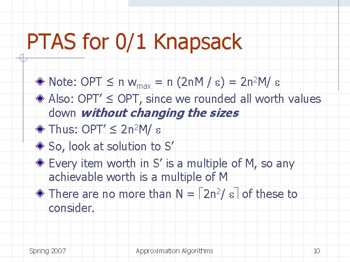
PTAS for 0/1 Knapsack Note: OPT ≤ n wmax = n (2 n. M / ) = 2 n 2 M/ Also: OPT’ ≤ OPT, since we rounded all worth values down without changing the sizes Thus: OPT’ ≤ 2 n 2 M/ So, look at solution to S’ Every item worth in S’ is a multiple of M, so any achievable worth is a multiple of M There are no more than N = 2 n 2/ of these to consider. Spring 2007 Approximation Algorithms 10

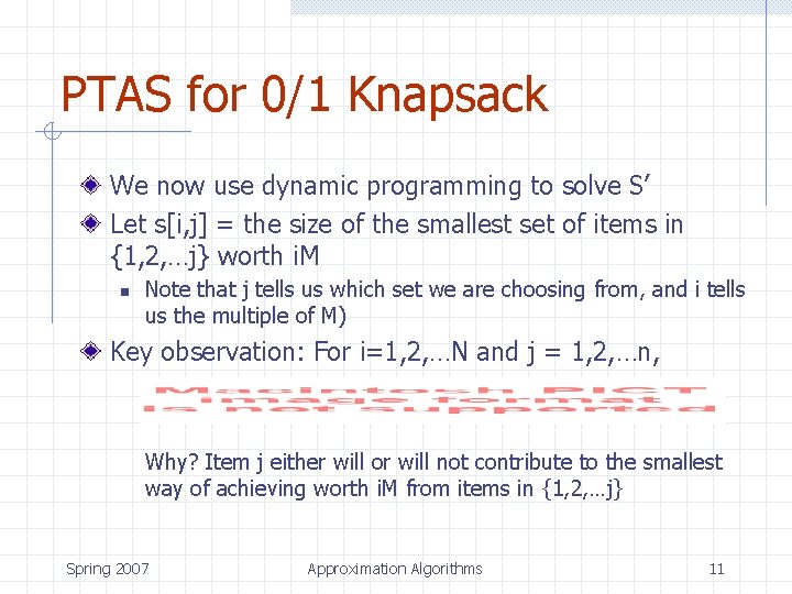
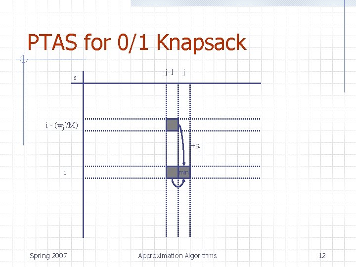
PTAS for 0/1 Knapsack We now use dynamic programming to solve S’ Let s[i, j] = the size of the smallest set of items in {1, 2, …j} worth i. M n Note that j tells us which set we are choosing from, and i tells us the multiple of M) Key observation: For i=1, 2, …N and j = 1, 2, …n, Why? Item j either will or will not contribute to the smallest way of achieving worth i. M from items in {1, 2, …j} Spring 2007 Approximation Algorithms 11

PTAS for 0/1 Knapsack s j-1 j i - (wj /M) +sj i Spring 2007 min Approximation Algorithms 12

PTAS for 0/1 Knapsack Define s[i, 0]=+ for i = 1, 2, …N n Roughly, no items implies we need infinitely many of them to achieve worth i. M Define s[0, j]=0 for j = 1, 2, …n Optimal value OPT’ = max{i. M: s[i, n]≤s} Cost of the algorithm O(n. N) = O(n 3/ ) Spring 2007 Approximation Algorithms 13

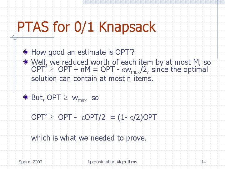
PTAS for 0/1 Knapsack How good an estimate is OPT’? Well, we reduced worth of each item by at most M, so OPT’ ≥ OPT – n. M = OPT - wmax/2, since the optimal solution can contain at most n items. But, OPT ≥ wmax so OPT’ ≥ OPT - OPT/2 = (1 - /2)OPT which is what we needed to prove. Spring 2007 Approximation Algorithms 14

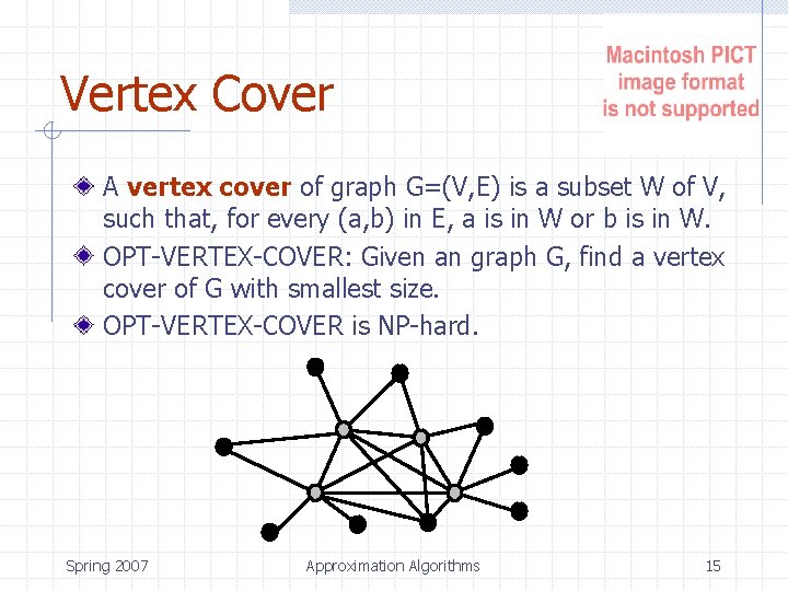
Vertex Cover A vertex cover of graph G=(V, E) is a subset W of V, such that, for every (a, b) in E, a is in W or b is in W. OPT-VERTEX-COVER: Given an graph G, find a vertex cover of G with smallest size. OPT-VERTEX-COVER is NP-hard. Spring 2007 Approximation Algorithms 15

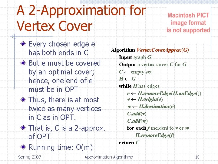
A 2 -Approximation for Vertex Cover Every chosen edge e has both ends in C But e must be covered by an optimal cover; hence, one end of e must be in OPT Thus, there is at most twice as many vertices in C as in OPT. That is, C is a 2 -approx. of OPT Running time: O(m) Spring 2007 Algorithm Vertex. Cover. Approx(G) Input graph G Output a vertex cover C for G C empty set H G while H has edges e H. remove. Edge(H. an. Edge()) v H. origin(e) w H. destination(e) C. add(v) C. add(w) for each f incident to v or w H. remove. Edge(f) return C Approximation Algorithms 16

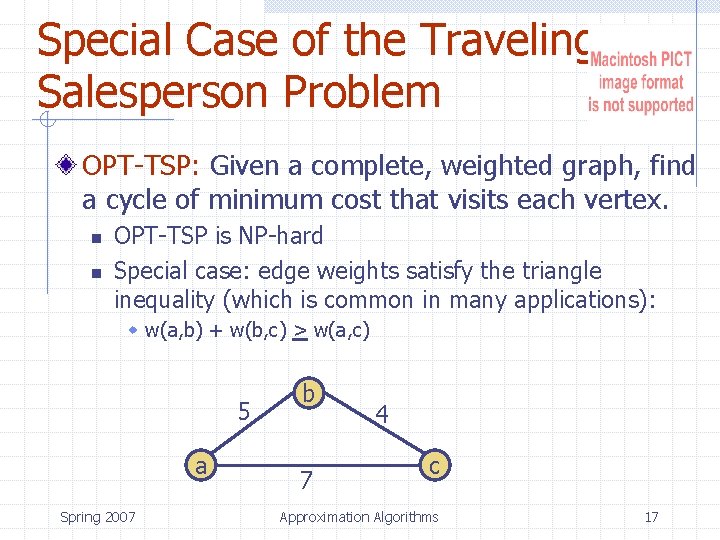
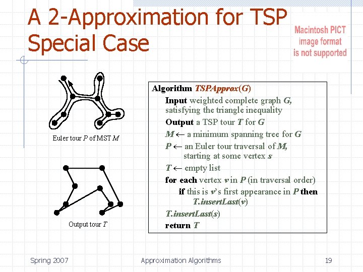
Special Case of the Traveling Salesperson Problem OPT-TSP: Given a complete, weighted graph, find a cycle of minimum cost that visits each vertex. n n OPT-TSP is NP-hard Special case: edge weights satisfy the triangle inequality (which is common in many applications): w w(a, b) + w(b, c) > w(a, c) 5 a Spring 2007 b 7 4 c Approximation Algorithms 17

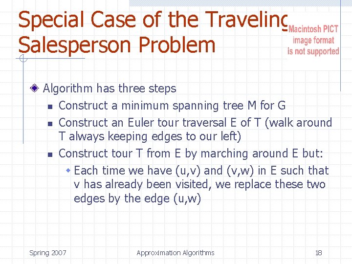
Special Case of the Traveling Salesperson Problem Algorithm has three steps n Construct a minimum spanning tree M for G n Construct an Euler tour traversal E of T (walk around T always keeping edges to our left) n Construct tour T from E by marching around E but: w Each time we have (u, v) and (v, w) in E such that v has already been visited, we replace these two edges by the edge (u, w) Spring 2007 Approximation Algorithms 18

A 2 -Approximation for TSP Special Case Euler tour P of MST M Output tour T Spring 2007 Algorithm TSPApprox(G) Input weighted complete graph G, satisfying the triangle inequality Output a TSP tour T for G M a minimum spanning tree for G P an Euler tour traversal of M, starting at some vertex s T empty list for each vertex v in P (in traversal order) if this is v’s first appearance in P then T. insert. Last(v) T. insert. Last(s) return T Approximation Algorithms 19

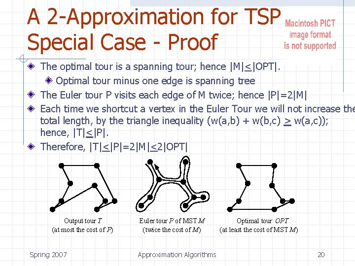
A 2 -Approximation for TSP Special Case - Proof The optimal tour is a spanning tour; hence |M|<|OPT|. Optimal tour minus one edge is spanning tree The Euler tour P visits each edge of M twice; hence |P|=2|M| Each time we shortcut a vertex in the Euler Tour we will not increase the total length, by the triangle inequality (w(a, b) + w(b, c) > w(a, c)); hence, |T|<|P|. Therefore, |T|<|P|=2|M|<2|OPT| Output tour T (at most the cost of P) Spring 2007 Euler tour P of MST M (twice the cost of M) Approximation Algorithms Optimal tour OPT (at least the cost of MST M) 20

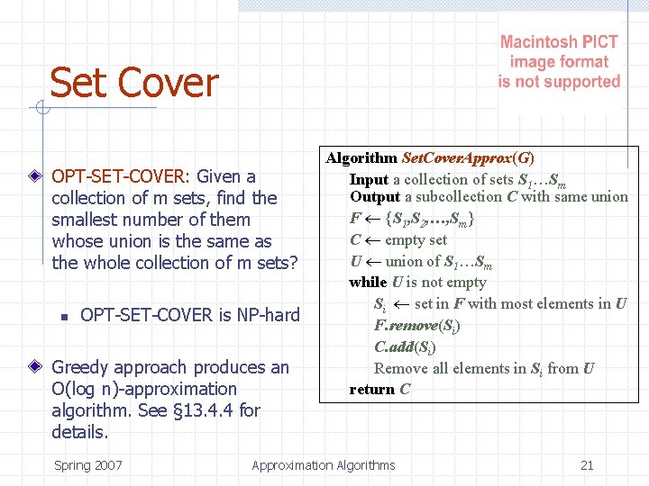
Set Cover OPT-SET-COVER: Given a collection of m sets, find the smallest number of them whose union is the same as the whole collection of m sets? n OPT-SET-COVER is NP-hard Greedy approach produces an O(log n)-approximation algorithm. See § 13. 4. 4 for details. Spring 2007 Algorithm Set. Cover. Approx(G) Input a collection of sets S 1…Sm Output a subcollection C with same union F {S 1, S 2, …, Sm} C empty set U union of S 1…Sm while U is not empty Si set in F with most elements in U F. remove(Si) C. add(Si) Remove all elements in Si from U return C Approximation Algorithms 21

Backtracking and -and-Bound Spring 2007 Approximation Algorithms Branch 22

Back to NP-Completeness Many hard problems are NP-Complete n But we still need solutions to them, even if they take a long time to generate Backtracking and Branch-and-Bound are two design techniques that have proven promising for dealing with NP-Complete problems n And often these find ``good enough’’ solutions in a reasonable amount of time Spring 2007 Approximation Algorithms 23

Backtracking A backtracking algorithm searches through a large set of possibilities in a systematic way n n Typically optimized to avoid symmetries in problem instances (think, e. g. , TSP) Traverses search space in manner such that ``easy’’ solution is found if one exists. Technique takes advantage of an inherent structure possessed by many NP-Complete problems Spring 2007 Approximation Algorithms 24

NP-Complete Problem Structure Recall: acceptance of solution for instance x of NP-complete problem can be verified in polynomial time Verification typically involves checking a set of choices (the output of the choice function) to see whether they satisfy a formula or demonstrate a successful configuration n E. g. , Values assigned to Boolean variables, vertices of graph to include in special set, items to go in knapsack Spring 2007 Approximation Algorithms 25

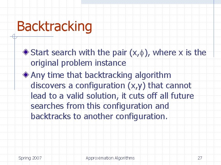
Backtracking Systematically searches for a solution to problem Traverses through possible ``search paths’’ to locate solutions or dead ends Configuration at end of such a path consists of a pair (x, y) n n x is the remaining problem to be solved y is the set of choices that have been made to get to this subproblem from the original problem instance Spring 2007 Approximation Algorithms 26

Backtracking Start search with the pair (x, ), where x is the original problem instance Any time that backtracking algorithm discovers a configuration (x, y) that cannot lead to a valid solution, it cuts off all future searches from this configuration and backtracks to another configuration. Spring 2007 Approximation Algorithms 27

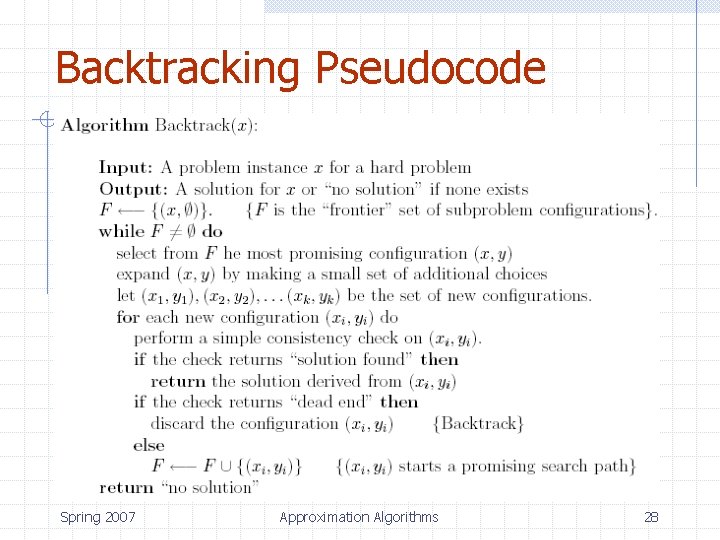
Backtracking Pseudocode Spring 2007 Approximation Algorithms 28

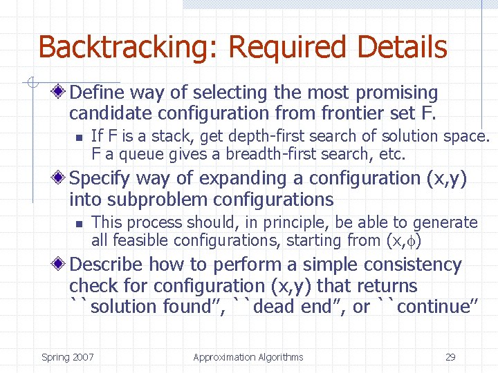
Backtracking: Required Details Define way of selecting the most promising candidate configuration from frontier set F. n If F is a stack, get depth-first search of solution space. F a queue gives a breadth-first search, etc. Specify way of expanding a configuration (x, y) into subproblem configurations n This process should, in principle, be able to generate all feasible configurations, starting from (x, ) Describe how to perform a simple consistency check for configuration (x, y) that returns ``solution found’’, ``dead end’’, or ``continue’’ Spring 2007 Approximation Algorithms 29

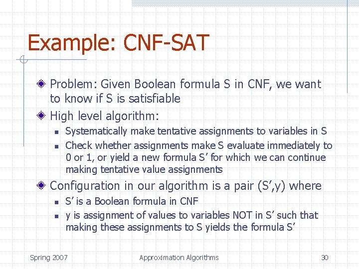
Example: CNF-SAT Problem: Given Boolean formula S in CNF, we want to know if S is satisfiable High level algorithm: n n Systematically make tentative assignments to variables in S Check whether assignments make S evaluate immediately to 0 or 1, or yield a new formula S’ for which we can continue making tentative value assignments Configuration in our algorithm is a pair (S’, y) where n n S’ is a Boolean formula in CNF y is assignment of values to variables NOT in S’ such that making these assignments to S yields the formula S’ Spring 2007 Approximation Algorithms 30

Example: CNF-SAT (details) Given frontier F of configurations, the most promising subproblem S’ is the one with the smallest clause n This formula would be the most constrained of all formulas in F, so we expect it to hit a dead end most quickly (if it’s going to hit a dead end) To generate new subproblem from S’, locate smallest clause in S’, pick a variable xi that appears in that clause, and create two new subproblems associated with assigning xi=0 and xi=1 respectively Spring 2007 Approximation Algorithms 31

Example: CNF-SAT (details) Processing S’ for consistency check for assignment of a variable xi in S’ n n n First, reduce any clauses containing xi based on the value assigned to xi If this reduction results in new single literal clause (xj or ~xj) we assign value to xj to make single literal clause satisfied. Repeat process until no single literal clauses If we discover a contradiction (clauses xi and ~xi , or an empty clause) we return ``dead end’’ If we reduce S’ all the way to constant 1, return ``solution found’’ along with assignments made to reach this Else, derive new subformula S’’ such that each clause has at least two literals, along with value assignments that lead from S to S’’ (this is the reduce operation) Spring 2007 Approximation Algorithms 32

Example: CNF-SAT (details) Placing this in backtracking template results in algorithm that has exponential worst case run time, but usually does OK In fact, if each clause has no more than two literals, this algorithm runs in polynomial time. Spring 2007 Approximation Algorithms 33

Branch-and-Bound Backtracking not designed for optimization problems, where in addition to having some feasibility condition that must be satisfied, we also have a cost f(x) to be optimized n We’ll assume minimized Can extend backtracking to work with optimization problems (result is Branch-and-Bound) n n When a solution is found, we continue processing to find the best solution Add a scoring mechanism to always choose most promising configuration to explore in each iteration (best-first search) Spring 2007 Approximation Algorithms 34

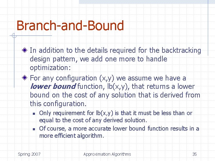
Branch-and-Bound In addition to the details required for the backtracking design pattern, we add one more to handle optimization: For any configuration (x, y) we assume we have a lower bound function, lb(x, y), that returns a lower bound on the cost of any solution that is derived from this configuration. n n Only requirement for lb(x, y) is that it must be less than or equal to the cost of any derived solution. Of course, a more accurate lower bound function results in a more efficient algorithm. Spring 2007 Approximation Algorithms 35

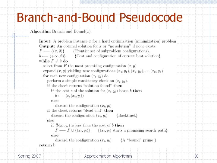
Branch-and-Bound Pseudocode Spring 2007 Approximation Algorithms 36

Branch-and-Bound Alg. for TSP Problem: optimization version of TSP n n Given weighted graph G, want least cost tour For edge e, let c(e) be the weight (cost) of edge e We compute, for each edge e = (v, w) in G, the minimum cost path that begins at v and ends at w while visiting all other vertices of G along the way We generate the path from v to w in G – {e} by augmenting a current path by one vertex in each loop of the branch-and-bound algorithm Spring 2007 Approximation Algorithms 37

Branch-and-Bound Alg. for TSP After having built a partial path P, starting, say, at v, we only consider augmenting P with vertices not in P We can classify a partial path P as a ``dead end’’ if the vertices not in P are disconnected in G – {e} We define the lower bound function to be the total cost of the edges in P plus c(e). n Certainly a lower bound for any tour built from e and P Spring 2007 Approximation Algorithms 38

Branch-and-Bound Alg. for TSP After having run the algorithm to completion for one edge of G, we can use the best path found so far over all tested edges, rather than restarting the current best solution b at + Run time can still be exponential, but we eliminate a considerable amount of redundancy There are other heuristics for approximating TSP. We won’t discuss them here. Spring 2007 Approximation Algorithms 39