Greedy vs Dynamic Programming Approach Comparing the methods

Greedy vs Dynamic Programming Approach • Comparing the methods • Knapsack problem • Greedy algorithms for 0/1 knapsack • An approximation algorithm for 0/1 knapsack • Optimal greedy algorithm for knapsack with fractions • A dynamic programming algorithm for 0/1 knapsack 1999 Cutler/Head

Greedy Approach VS Dynamic Programming (DP) • Greedy and Dynamic Programming are methods for solving optimization problems. • Greedy algorithms are usually more efficient than DP solutions. • However, often you need to use dynamic programming since the optimal solution cannot be guaranteed by a greedy algorithm. • DP provides efficient solutions for some problems for which a brute force approach would be very slow. • To use Dynamic Programming we need only show that the principle of optimality applies to the problem. 1999 Cutler/Head 2

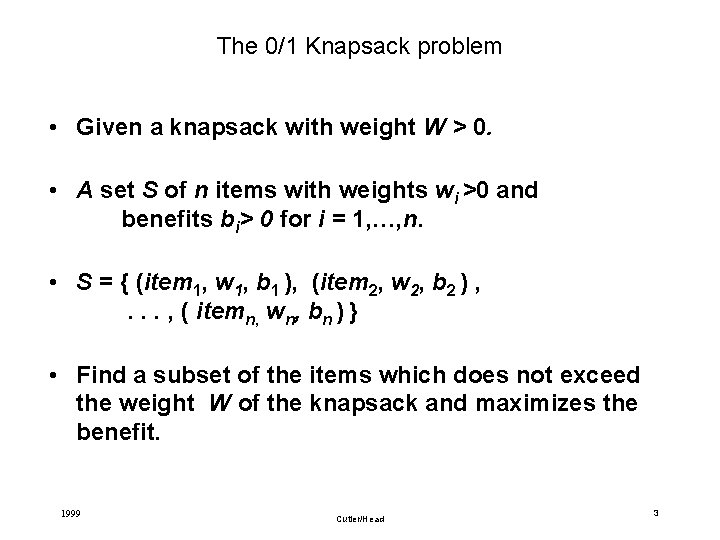
The 0/1 Knapsack problem • Given a knapsack with weight W > 0. • A set S of n items with weights wi >0 and benefits bi> 0 for i = 1, …, n. • S = { (item 1, w 1, b 1 ), (item 2, w 2, b 2 ) , . . . , ( itemn, wn, bn ) } • Find a subset of the items which does not exceed the weight W of the knapsack and maximizes the benefit. 1999 Cutler/Head 3

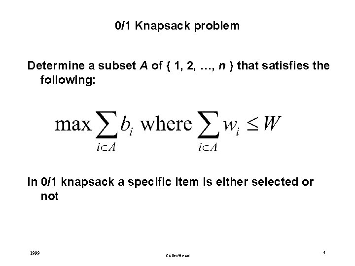
0/1 Knapsack problem Determine a subset A of { 1, 2, …, n } that satisfies the following: In 0/1 knapsack a specific item is either selected or not 1999 Cutler/Head 4

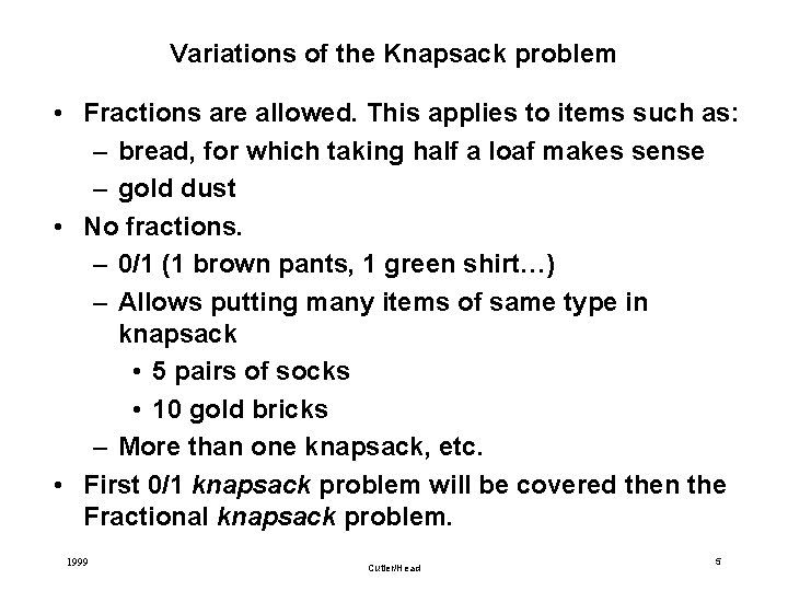
Variations of the Knapsack problem • Fractions are allowed. This applies to items such as: – bread, for which taking half a loaf makes sense – gold dust • No fractions. – 0/1 (1 brown pants, 1 green shirt…) – Allows putting many items of same type in knapsack • 5 pairs of socks • 10 gold bricks – More than one knapsack, etc. • First 0/1 knapsack problem will be covered then the Fractional knapsack problem. 1999 Cutler/Head 5

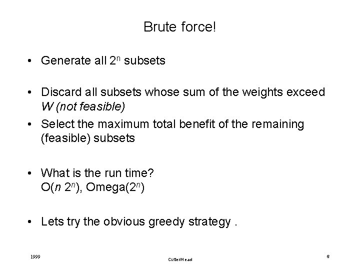
Brute force! • Generate all 2 n subsets • Discard all subsets whose sum of the weights exceed W (not feasible) • Select the maximum total benefit of the remaining (feasible) subsets • What is the run time? O(n 2 n), Omega(2 n) • Lets try the obvious greedy strategy. 1999 Cutler/Head 6

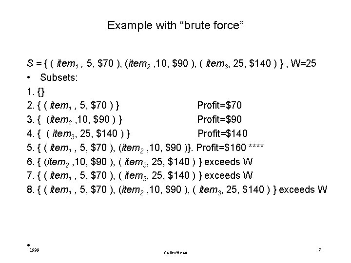
Example with “brute force” S = { ( item 1 , 5, $70 ), (item 2 , 10, $90 ), ( item 3, 25, $140 ) } , W=25 • Subsets: 1. {} 2. { ( item 1 , 5, $70 ) } Profit=$70 3. { (item 2 , 10, $90 ) } Profit=$90 4. { ( item 3, 25, $140 ) } Profit=$140 5. { ( item 1 , 5, $70 ), (item 2 , 10, $90 )}. Profit=$160 **** 6. { (item 2 , 10, $90 ), ( item 3, 25, $140 ) } exceeds W 7. { ( item 1 , 5, $70 ), ( item 3, 25, $140 ) } exceeds W 8. { ( item 1 , 5, $70 ), (item 2 , 10, $90 ), ( item 3, 25, $140 ) } exceeds W • 1999 Cutler/Head 7

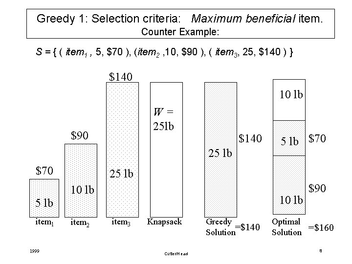
Greedy 1: Selection criteria: Maximum beneficial item. Counter Example: S = { ( item 1 , 5, $70 ), (item 2 , 10, $90 ), ( item 3, 25, $140 ) } $140 10 lb W= 25 lb $90 $140 25 lb $70 25 lb 10 lb 5 lb item 1 1999 5 lb $70 item 2 item 3 Knapsack Cutler/Head Greedy =$140 Solution $90 Optimal Solution =$160 8

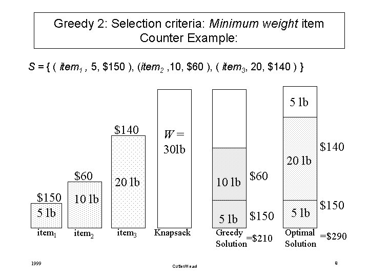
Greedy 2: Selection criteria: Minimum weight item Counter Example: S = { ( item 1 , 5, $150 ), (item 2 , 10, $60 ), ( item 3, 20, $140 ) } 5 lb $140 $60 $150 5 lb 10 lb item 1 item 2 1999 W= 30 lb $140 20 lb 10 lb $60 20 lb 5 lb $150 item 3 Knapsack Cutler/Head Greedy =$210 Solution 5 lb $150 Optimal =$290 Solution 9

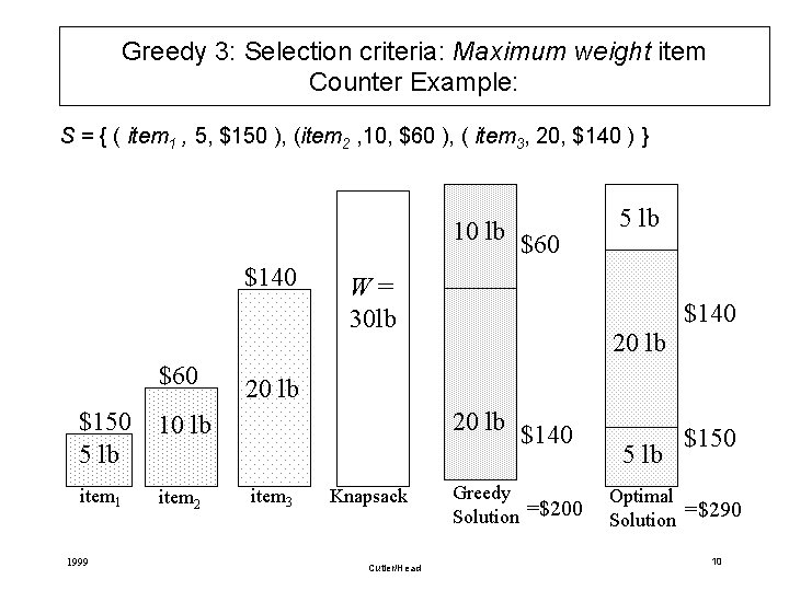
Greedy 3: Selection criteria: Maximum weight item Counter Example: S = { ( item 1 , 5, $150 ), (item 2 , 10, $60 ), ( item 3, 20, $140 ) } 10 lb $60 $140 $60 $150 5 lb 10 lb item 1 item 2 1999 W= 30 lb 5 lb $140 20 lb $140 item 3 Knapsack Cutler/Head Greedy Solution =$200 5 lb $150 Optimal Solution =$290 10

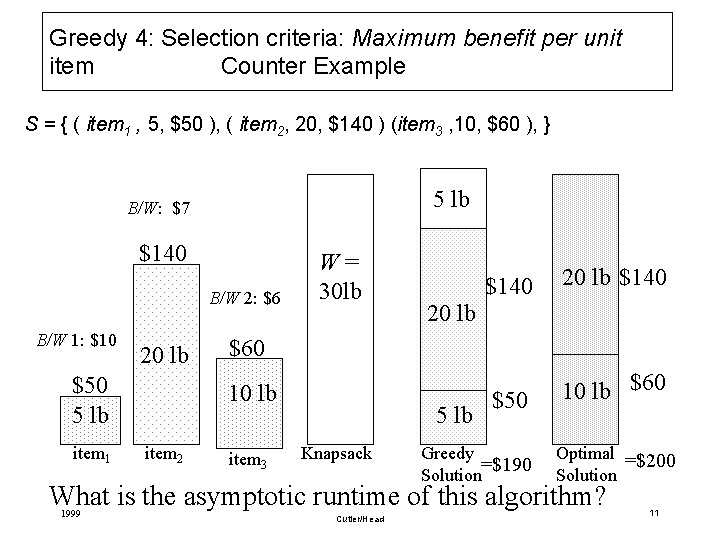
Greedy 4: Selection criteria: Maximum benefit per unit item Counter Example S = { ( item 1 , 5, $50 ), ( item 2, 20, $140 ) (item 3 , 10, $60 ), } 5 lb B/W: $7 $140 B/W 2: $6 B/W 1: $10 20 lb $50 5 lb item 1 W= 30 lb 20 lb $140 $50 10 lb $60 20 lb $60 10 lb item 2 $140 item 3 5 lb Knapsack Greedy =$190 Solution Optimal =$200 Solution What is the asymptotic runtime of this algorithm? 1999 Cutler/Head 11

Approximation algorithms • Approximation algorithms attempt to evaluate how far away from the optimum OPT, are the solutions sol. Alg provided by an algorithm in the worst case • Many criteria are used. We use OPT/sol. Alg for maximization, and attempt to establish OPT/sol. Alg<=K where K is a constant (sol. Alg/OPT for minimization) • The following slides show that the “best” greedy algorithm for 0/1 knapsack, greedy 4 does not satisfy OPT/sol. Alg<=K • Often greedy 4 gives an optimal solutions, but for some problem instances the ratio can become very large • A small modification of greedy 4, however, guarantees, that OPT/alg<=2 • This is a big improvement. • There are better approximation algorithms for knapsack 1999 Cutler/Head 12

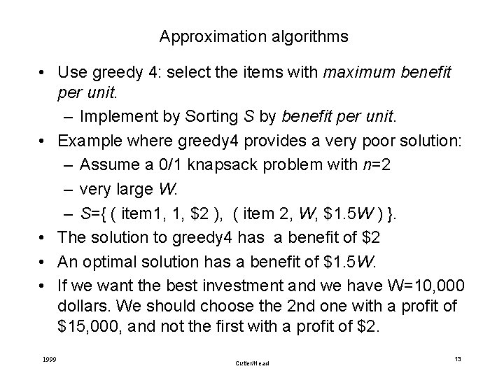
Approximation algorithms • Use greedy 4: select the items with maximum benefit per unit. – Implement by Sorting S by benefit per unit. • Example where greedy 4 provides a very poor solution: – Assume a 0/1 knapsack problem with n=2 – very large W. – S={ ( item 1, 1, $2 ), ( item 2, W, $1. 5 W ) }. • The solution to greedy 4 has a benefit of $2 • An optimal solution has a benefit of $1. 5 W. • If we want the best investment and we have W=10, 000 dollars. We should choose the 2 nd one with a profit of $15, 000, and not the first with a profit of $2. 1999 Cutler/Head 13

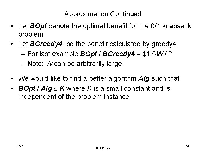
Approximation Continued • Let BOpt denote the optimal benefit for the 0/1 knapsack problem • Let BGreedy 4 be the benefit calculated by greedy 4. – For last example BOpt / BGreedy 4 = $1. 5 W / 2 – Note: W can be arbitrarily large • We would like to find a better algorithm Alg such that • BOpt / Alg K where K is a small constant and is independent of the problem instance. 1999 Cutler/Head 14

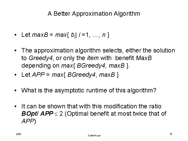
A Better Approximation Algorithm • Let max. B = max{ bi| i =1, …, n } • The approximation algorithm selects, either the solution to Greedy 4, or only the item with benefit Max. B depending on max{ BGreedy 4, max. B }. • Let APP = max{ BGreedy 4, max. B } • What is the asymptotic runtime of this algorithm? • It can be shown that with this modification the ratio BOpt/ APP 2 (Optimal benefit at most twice that of APP) 1999 Cutler/Head 15

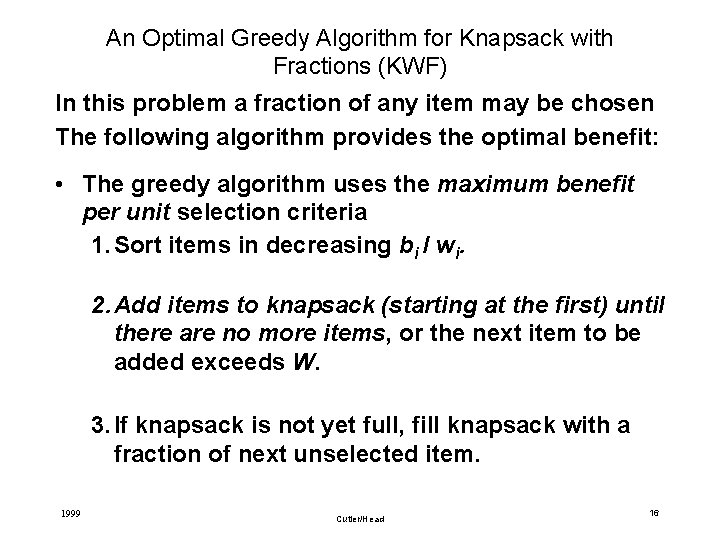
An Optimal Greedy Algorithm for Knapsack with Fractions (KWF) In this problem a fraction of any item may be chosen The following algorithm provides the optimal benefit: • The greedy algorithm uses the maximum benefit per unit selection criteria 1. Sort items in decreasing bi / wi. 2. Add items to knapsack (starting at the first) until there are no more items, or the next item to be added exceeds W. 3. If knapsack is not yet full, fill knapsack with a fraction of next unselected item. 1999 Cutler/Head 16

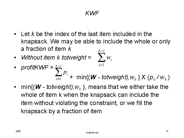
KWF • Let k be the index of the last item included in the knapsack. We may be able to include the whole or only a fraction of item k • Without item k totweight = • profit. KWF = + min{(W - totweight), wk } X (pk / wk ) • min{(W - totweight), wk }, means that we either take the whole of item k when the knapsack can include the item without violating the constraint, or we fill the knapsack by a fraction of item 1999 Cutler/Head 17

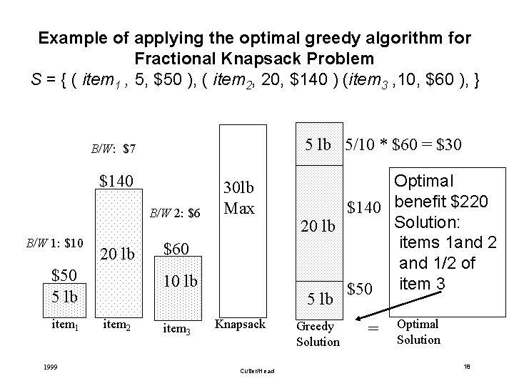
Example of applying the optimal greedy algorithm for Fractional Knapsack Problem S = { ( item 1 , 5, $50 ), ( item 2, 20, $140 ) (item 3 , 10, $60 ), } 5 lb 5/10 * $60 = $30 B/W: $7 $140 B/W 2: $6 B/W 1: $10 20 lb $50 5 lb item 1 1999 30 lb Max $60 10 lb item 2 item 3 Knapsack Cutler/Head Optimal $140 benefit $220 Solution: 20 lb items 1 and 2 and 1/2 of item 3 $50 5 lb Greedy Solution = Optimal Solution 18

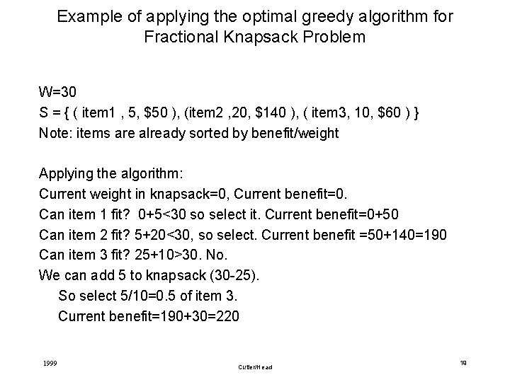
Example of applying the optimal greedy algorithm for Fractional Knapsack Problem W=30 S = { ( item 1 , 5, $50 ), (item 2 , 20, $140 ), ( item 3, 10, $60 ) } Note: items are already sorted by benefit/weight Applying the algorithm: Current weight in knapsack=0, Current benefit=0. Can item 1 fit? 0+5<30 so select it. Current benefit=0+50 Can item 2 fit? 5+20<30, so select. Current benefit =50+140=190 Can item 3 fit? 25+10>30. No. We can add 5 to knapsack (30 -25). So select 5/10=0. 5 of item 3. Current benefit=190+30=220 1999 Cutler/Head 19

Greedy Algorithm for Knapsack with fractions • To show that the greedy algorithm finds the optimal profit for the fractional Knapsack problem you need to prove there is no solution with a higher profit (see text) • Notice there may be more than one optimal solution 1999 Cutler/Head 20

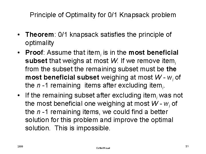
Principle of Optimality for 0/1 Knapsack problem • Theorem: 0/1 knapsack satisfies the principle of optimality • Proof: Assume that itemi is in the most beneficial subset that weighs at most W. If we remove itemi from the subset the remaining subset must be the most beneficial subset weighing at most W - wi of the n -1 remaining items after excluding itemi. • If the remaining subset after excluding itemi was not the most beneficial one weighing at most W - wi of the n -1 remaining items, we could find a better solution for this problem and improve the optimal solution. This is impossible. 1999 Cutler/Head 21

Dynamic Programming Approach • Given a knapsack problem with n items and knapsack weight of W. • We will first compute the maximum benefit, and then determine the subset. • To use dynamic programming we solve smaller problems and use the optimal solutions of these problems to find the solution to larger ones. 1999 Cutler/Head 22

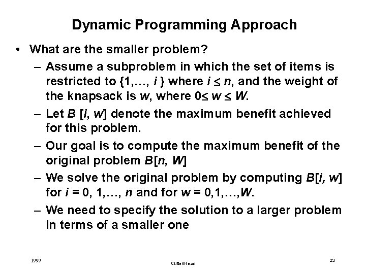
Dynamic Programming Approach • What are the smaller problem? – Assume a subproblem in which the set of items is restricted to {1, …, i } where i n, and the weight of the knapsack is w, where 0 w W. – Let B [i, w] denote the maximum benefit achieved for this problem. – Our goal is to compute the maximum benefit of the original problem B[n, W] – We solve the original problem by computing B[i, w] for i = 0, 1, …, n and for w = 0, 1, …, W. – We need to specify the solution to a larger problem in terms of a smaller one 1999 Cutler/Head 23

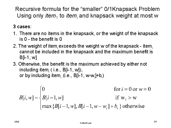
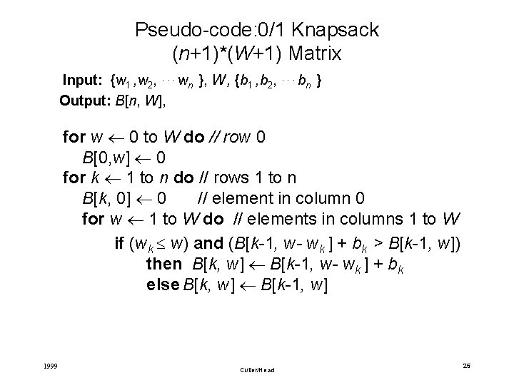
Recursive formula for the “smaller” 0/1 Knapsack Problem Using only item 1 to itemi and knapsack weight at most w 3 cases: 1. There are no items in the knapsack, or the weight of the knapsack is 0 - the benefit is 0 2. The weight of itemi exceeds the weight w of the knapsack - itemi cannot be included in the knapsack and the maximum benefit is B[i-1, w] 3. Otherwise, the benefit is the maximum achieved by either not including itemi ( i. e. , B[i-1, w]), or by including itemi (i. e. , B[i-1, w-wi]+bi) 1999 Cutler/Head 24

Pseudo-code: 0/1 Knapsack (n+1)*(W+1) Matrix Input: {w 1 , w 2, . . . wn }, W , {b 1 , b 2, Output: B[n, W], . . . b n } for w 0 to W do // row 0 B[0, w] 0 for k 1 to n do // rows 1 to n B[k, 0] 0 // element in column 0 for w 1 to W do // elements in columns 1 to W if (wk w) and (B[k-1, w- wk ] + bk > B[k-1, w]) then B[k, w] B[k-1, w- wk ] + bk else B[k, w] B[k-1, w] 1999 Cutler/Head 25

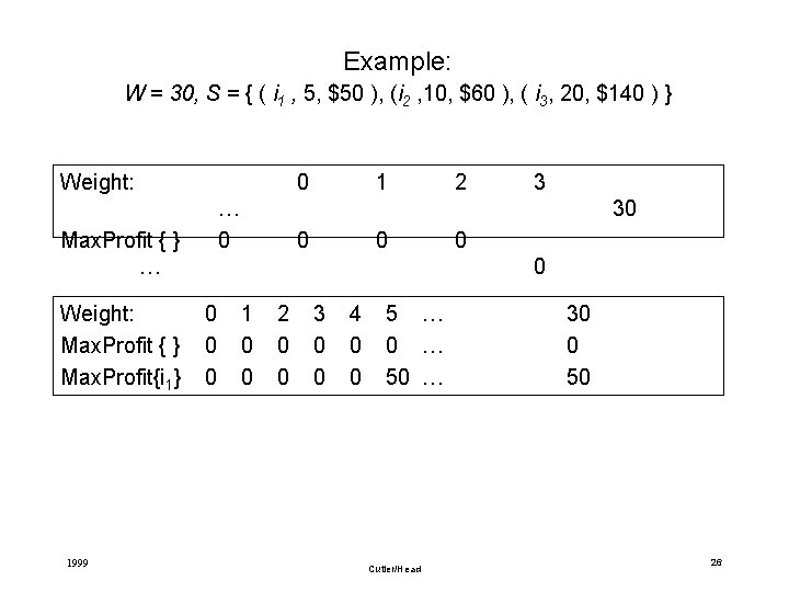
Example: W = 30, S = { ( i 1 , 5, $50 ), (i 2 , 10, $60 ), ( i 3, 20, $140 ) } Weight: 0 … 0 Max. Profit { } … Weight: Max. Profit { } Max. Profit{i 1} 1999 1 2 3 30 0 0 0 1 0 0 2 0 0 3 0 0 4 0 0 5 … 0 … 50 … Cutler/Head 30 0 50 26

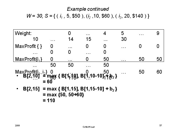
Example continued W = 30, S = { ( i 1 , 5, $50 ), (i 2 , 10, $60 ), ( i 3, 20, $140 ) } Weight: 0. . . 4 10 … 14 15. . . Max. Profit { } 0. . . 0 0 … 0 Max. Profit{i 1} 0. . . 0 50. . . 50 50 … 50 Max. Profit{i 1, i 2} 0 … 0 50 • B[2, 10] + b 2 } … = max 60 { B[1, 10], 110 B[1, 10 -10] … 110 = 60 • B[2, 15] = max { B[1, 15], B[1, 15 -10] + b 2 } = max {50, 50+60} = 110 1999 Cutler/Head 5 30 … … 9 0 0 … 50 50 … 50 60 27

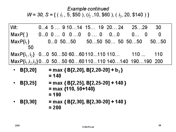
Example continued W = 30, S = { ( i 1 , 5, $50 ), (i 2 , 10, $60 ), ( i 3, 20, $140 ) } Wt: 0. . . 4 5 … 9 10… 14 15… 19 20… 24 25… 29 30 Max. P{ } 0. . . 0 0 … 0 0… 0 0 Max. P{i 1} 0. . . 0 50… 50 50… 50 50 Max. P{i 1, i 2} 0… 0 50… 50 60… 60 110. . . 110… 110. . . 110 Max. P{i 1, i 2, i 3} 0… 0 50… 50 60… 60 110. . . 110 140… 140 190… 190 200 • B[3, 20] • B[3, 25] • B[3, 30] 1999 = max { B[2, 20], B[2, 20 -20] + b 3 } = 140 = max { B[2, 25], B[2, 25 -20] + 140 } = max {110, 50+140} = 190 = max { B[2, 30], B[2, 30 -20] + 140 } = 200 Cutler/Head 28

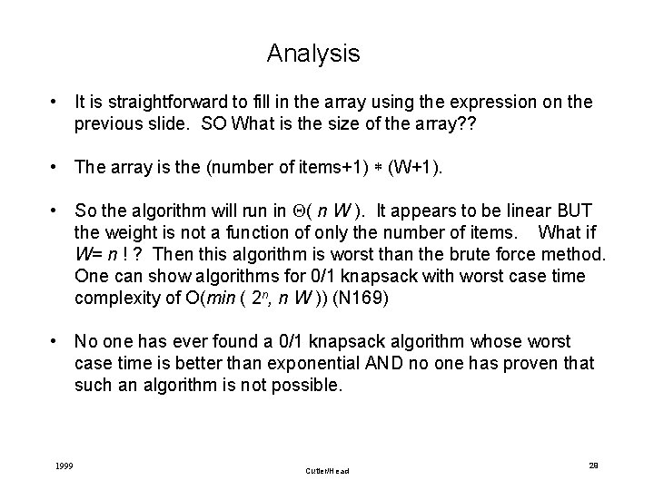
Analysis • It is straightforward to fill in the array using the expression on the previous slide. SO What is the size of the array? ? • The array is the (number of items+1) (W+1). • So the algorithm will run in ( n W ). It appears to be linear BUT the weight is not a function of only the number of items. What if W= n ! ? Then this algorithm is worst than the brute force method. One can show algorithms for 0/1 knapsack with worst case time complexity of O(min ( 2 n, n W )) (N 169) • No one has ever found a 0/1 knapsack algorithm whose worst case time is better than exponential AND no one has proven that such an algorithm is not possible. 1999 Cutler/Head 29

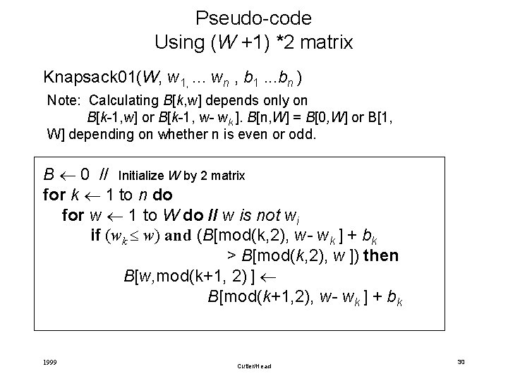
Pseudo-code Using (W +1) *2 matrix Knapsack 01(W, w 1, . . . wn , b 1. . . bn ) Note: Calculating B[k, w] depends only on B[k-1, w] or B[k-1, w- wk ]. B[n, W] = B[0, W] or B[1, W] depending on whether n is even or odd. B 0 // Initialize W by 2 matrix for k 1 to n do for w 1 to W do // w is not wi if (wk w) and (B[mod(k, 2), w- wk ] + bk > B[mod(k, 2), w ]) then B[w, mod(k+1, 2) ] B[mod(k+1, 2), w- wk ] + bk 1999 Cutler/Head 30