New algorithm for ADC INLDNL Test with ramp

New algorithm for ADC INL/DNL Test with ramp input Degang Chen 1

Basic assumptions and concepts 2

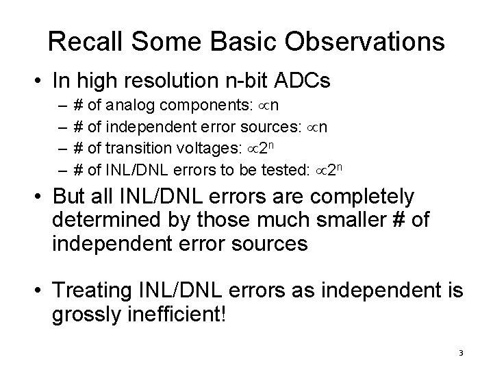
Recall Some Basic Observations • In high resolution n-bit ADCs – – # of analog components: n # of independent error sources: n # of transition voltages: 2 n # of INL/DNL errors to be tested: 2 n • But all INL/DNL errors are completely determined by those much smaller # of independent error sources • Treating INL/DNL errors as independent is grossly inefficient! 3

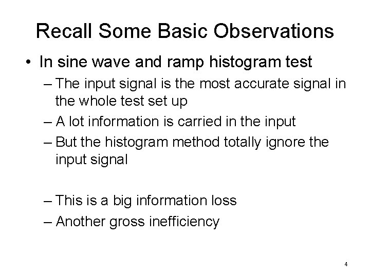
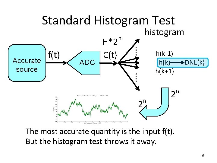
Recall Some Basic Observations • In sine wave and ramp histogram test – The input signal is the most accurate signal in the whole test set up – A lot information is carried in the input – But the histogram method totally ignore the input signal – This is a big information loss – Another gross inefficiency 4

Recall Some Basic Observations • For high resolution ADCs – Most of the errors are made by the first few MSB bits – Lower bits’ linearity performance is typically very good (after correction of some systematic errors) • Histogram test ignore this fact, another inefficiency • The lower bits can be used to “move samples” together for better noise averaging 5

Standard Histogram Test Accurate source f(t) ADC H*2 n C(t) histogram ⁞ h(k-1) h(k+1) ⁞ 2 n 2 DNL(k) n The most accurate quantity is the input f(t). But the histogram test throws it away. 6

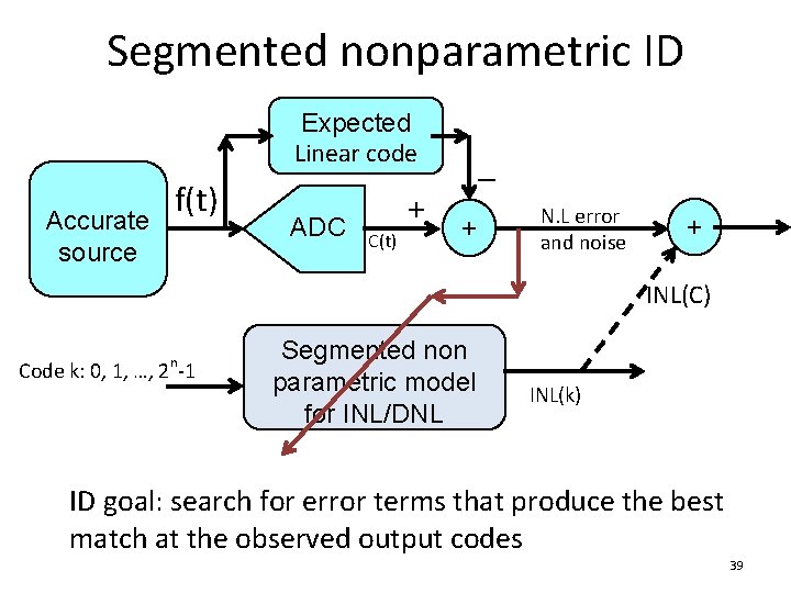
Segmented nonparametric ID Expected Linear code Accurate source f(t) ADC C(t) + – + N. L error and noise + INL(C) n Code k: 0, 1, …, 2 -1 Segmented non parametric model for INL/DNL INL(k) ID goal: search for error terms that produce the best match at the observed output codes 7

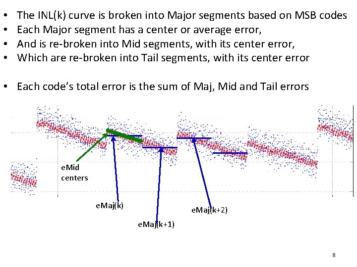
• • The INL(k) curve is broken into Major segments based on MSB codes Each Major segment has a center or average error, And is re-broken into Mid segments, with its center error, Which are re-broken into Tail segments, with its center error • Each code’s total error is the sum of Maj, Mid and Tail errors e. Mid centers e. Maj(k) e. Maj(k+2) e. Maj(k+1) 8

Notes • It is critical for each Maj segment not to involve major carrier transitions group by MSB codes • If lower bits (Mid and Tail) are reasonably linear, their errors within one Maj segment cancel out in computing Maj segment center errors, providing good accuracy in Maj segment centers • If not the case, systematic errors in lower bits can and should be tested and removed 9

Notes • Maj segment center locations capture true nonlinearities caused by voltage coefficients • For better capture of such nonlinearities, sufficient number of Maj segments are needed • Use a minimum of 4 or n/3 bits, whichever is larger, for Maj bits • But need a sufficient number of samples in each Maj segment for noise averaging • The above two are conflicting, tradeoff • But difficult for low resolution ADCs 10

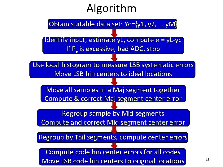
Algorithm Obtain suitable data set: Yc={y 1, y 2, … y. M} Identify input, estimate y. L, compute e = y. L-yc If Pe is excessive, bad ADC, stop Use local histogram to measure LSB systematic errors Move LSB bin centers to ideal locations Move all samples in a Maj segment together Compute & correct Maj segment center error Regroup sample by Mid segments Compute and correct Mid segment center error Regroup by Tail segments, compute center errors Compute code bin center errors for all codes Move LSB code bin centers to original locations 11

Removing LSB systematic errors 12

Why LSB bit systematic errors • Take a 16 -bit CDAC based SAR ADC as example • One popular lay out strategy: – 6 -bit MSB array, with 64 unit caps grouped into 6 -bit groups using 63 units, place dummy caps of ½ unit size around array. – The one left-over unit in parallel with some extra cap will make the bridge cap – Repeat the same array, for bit 7 to bit 12, the left-over bit can be used as redundant bit for dynamic error correction – Use one dummy as bit 13, split a dummy and use half as bit 14, split another dummy connecting in series as bit 15, split two dummies connecting ins eries as bit 16 • Bit 7 -12 will be super good; bit 13 not as good, bit 14 to bit 16 even worse, systematic errors 13

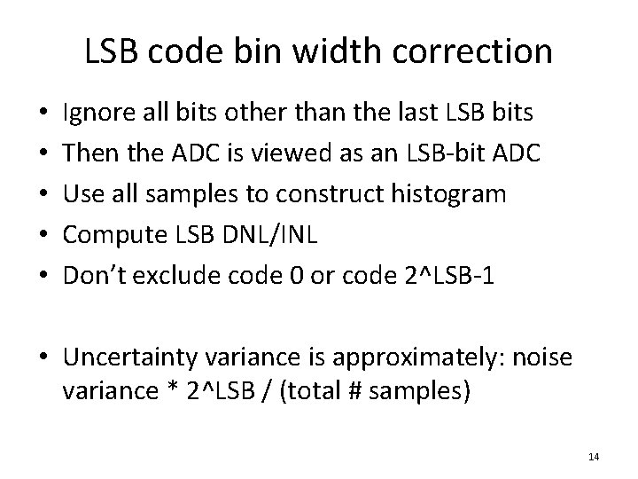
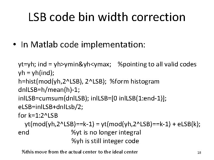
LSB code bin width correction • • • Ignore all bits other than the last LSB bits Then the ADC is viewed as an LSB-bit ADC Use all samples to construct histogram Compute LSB DNL/INL Don’t exclude code 0 or code 2^LSB-1 • Uncertainty variance is approximately: noise variance * 2^LSB / (total # samples) 14

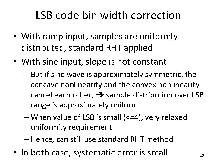
LSB code bin width correction • With ramp input, samples are uniformly distributed, standard RHT applied • With sine input, slope is not constant – But if sine wave is approximately symmetric, the concave nonlinearity and the convex nonlinearity cancel each other, sample distribution over LSB range is approximately uniform – When value of LSB is small (<=4), very relaxed uniformity requirement – Hence, can still use standard RHT method • In both case, systematic error is small 15

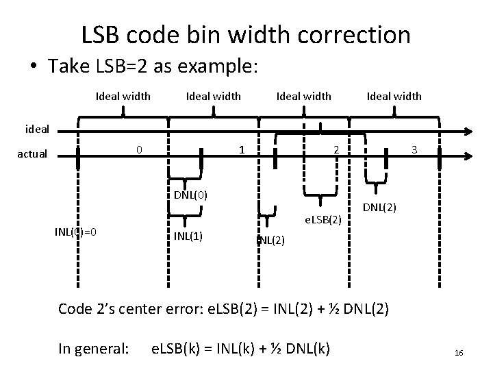
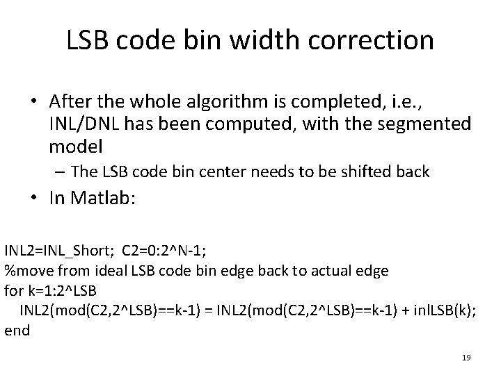
LSB code bin width correction • Take LSB=2 as example: Ideal width ideal 0 actual 1 2 DNL(0) INL(0)=0 e. LSB(2) INL(1) 3 DNL(2) INL(2) Code 2’s center error: e. LSB(2) = INL(2) + ½ DNL(2) In general: e. LSB(k) = INL(k) + ½ DNL(k) 16

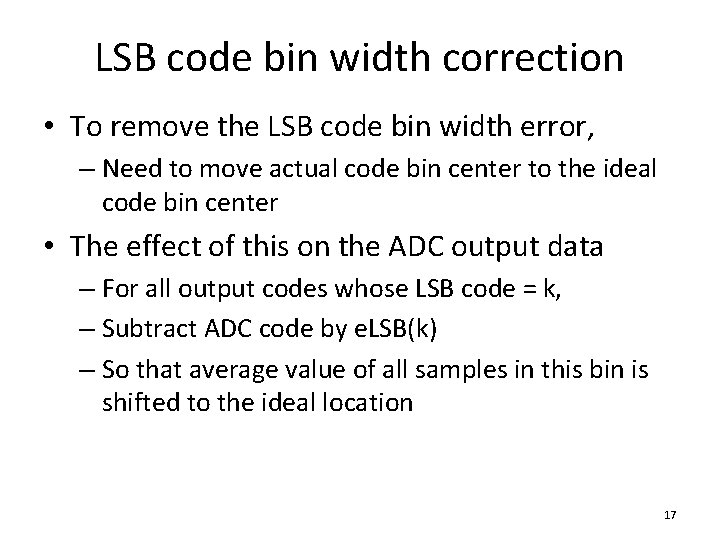
LSB code bin width correction • To remove the LSB code bin width error, – Need to move actual code bin center to the ideal code bin center • The effect of this on the ADC output data – For all output codes whose LSB code = k, – Subtract ADC code by e. LSB(k) – So that average value of all samples in this bin is shifted to the ideal location 17

LSB code bin width correction • In Matlab code implementation: yt=yh; ind = yh>ymin&yh<ymax; %pointing to all valid codes yh = yh(ind); h=hist(mod(yh, 2^LSB); %form histogram dnl. LSB=h/mean(h)-1; inl. LSB=cumsum(dnl. LSB); inl. LSB=[0 inl. LSB(1: end-1)]; e. LSB=inl. LSB+dnl. Lsb/2; for k=1: 2^LSB yt(mod(yh, 2^LSB)==k-1) = yt(mod(yh, 2^LSB)==k-1) + e. LSB(k); end %yt is no longer integral %yh is still integer code %this move from the actual center to the ideal center 18

LSB code bin width correction • After the whole algorithm is completed, i. e. , INL/DNL has been computed, with the segmented model – The LSB code bin center needs to be shifted back • In Matlab: INL 2=INL_Short; C 2=0: 2^N-1; %move from ideal LSB code bin edge back to actual edge for k=1: 2^LSB INL 2(mod(C 2, 2^LSB)==k-1) = INL 2(mod(C 2, 2^LSB)==k-1) + inl. LSB(k); end 19

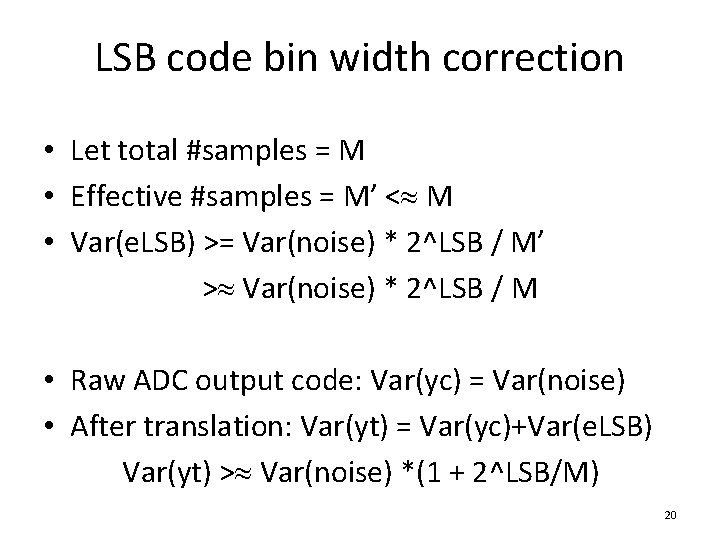
LSB code bin width correction • Let total #samples = M • Effective #samples = M’ < M • Var(e. LSB) >= Var(noise) * 2^LSB / M’ > Var(noise) * 2^LSB / M • Raw ADC output code: Var(yc) = Var(noise) • After translation: Var(yt) = Var(yc)+Var(e. LSB) Var(yt) > Var(noise) *(1 + 2^LSB/M) 20

Estimating output of a linear ADC and nonlinear error of actual ADC 21

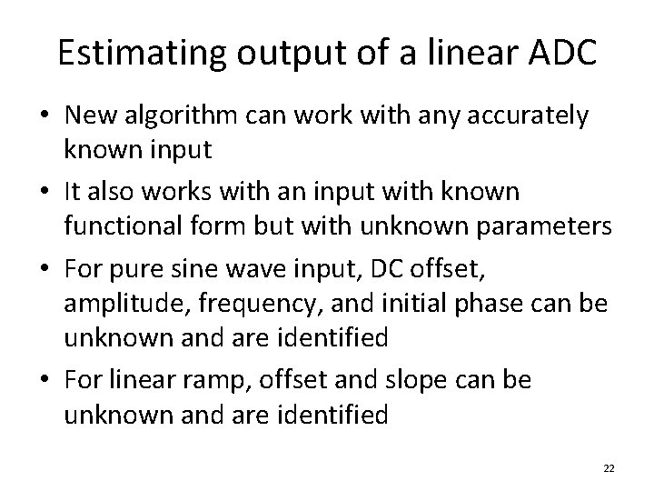
Estimating output of a linear ADC • New algorithm can work with any accurately known input • It also works with an input with known functional form but with unknown parameters • For pure sine wave input, DC offset, amplitude, frequency, and initial phase can be unknown and are identified • For linear ramp, offset and slope can be unknown and are identified 22

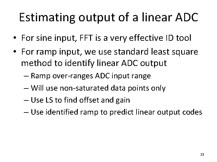
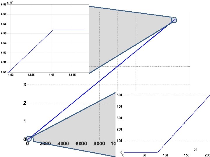
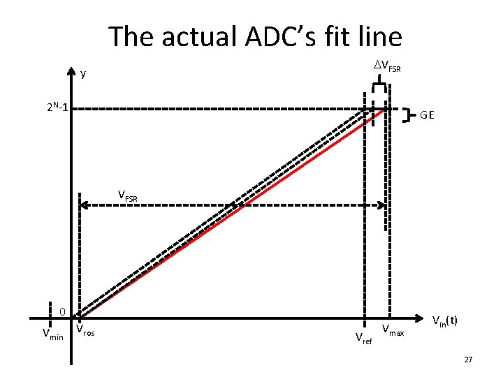
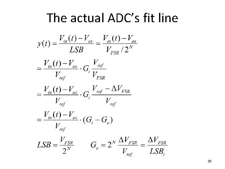
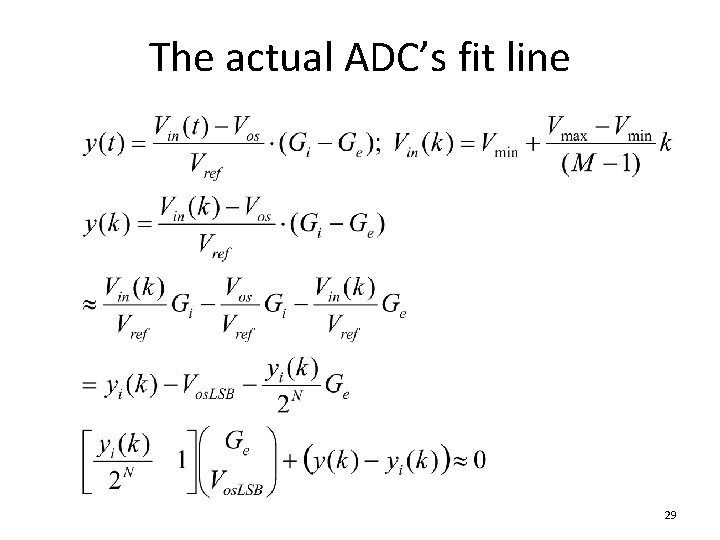
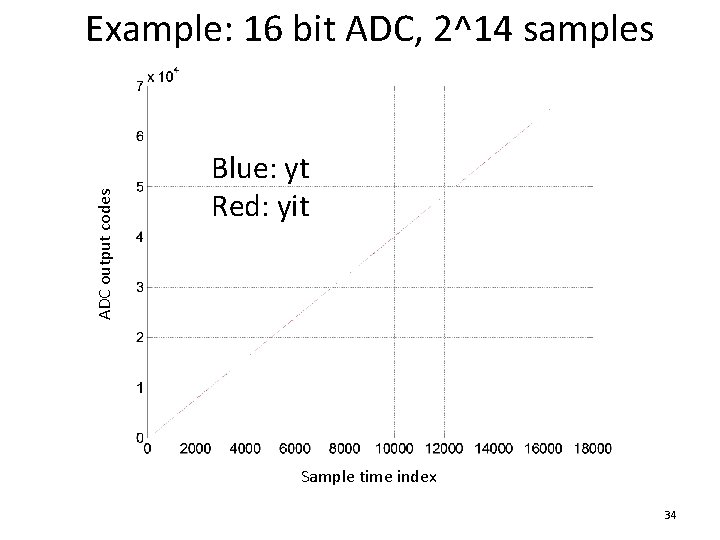
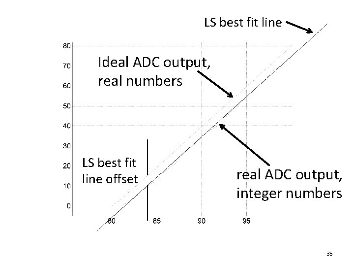
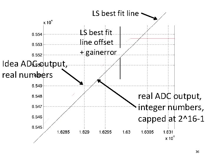
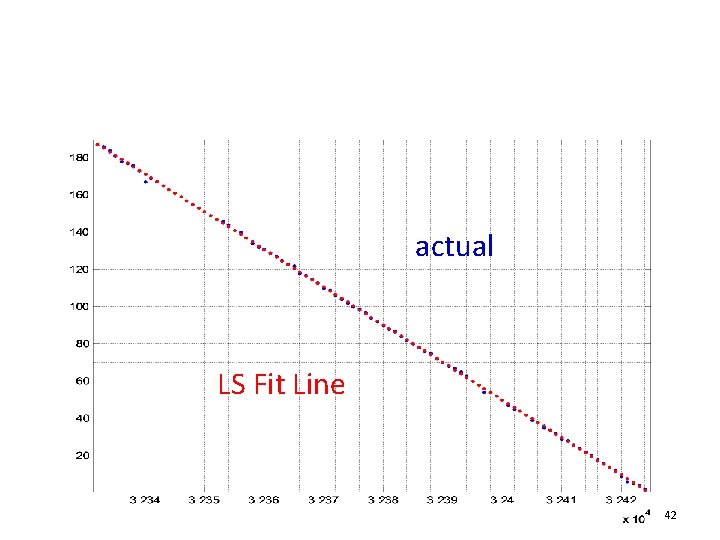
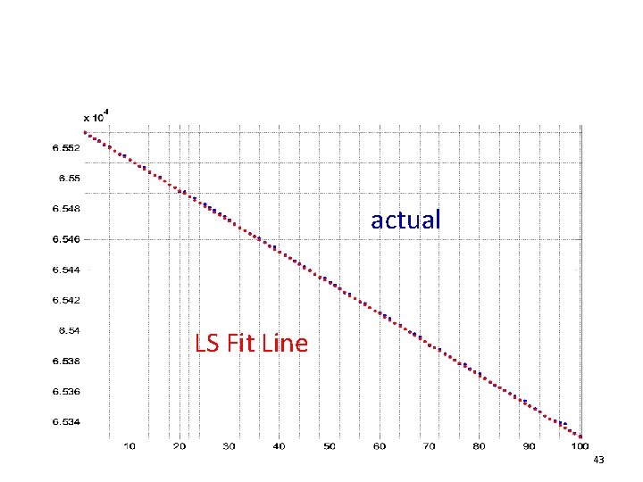
Estimating output of a linear ADC • For sine input, FFT is a very effective ID tool • For ramp input, we use standard least square method to identify linear ADC output – Ramp over-ranges ADC input range – Will use non-saturated data points only – Use LS to find offset and gain – Use identified ramp to predict linear output codes 23

24

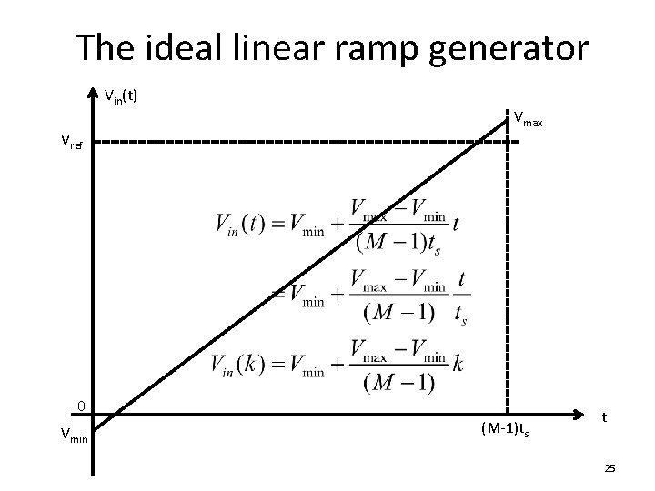
The ideal linear ramp generator Vin(t) Vmax Vref 0 Vmin (M-1)ts t 25

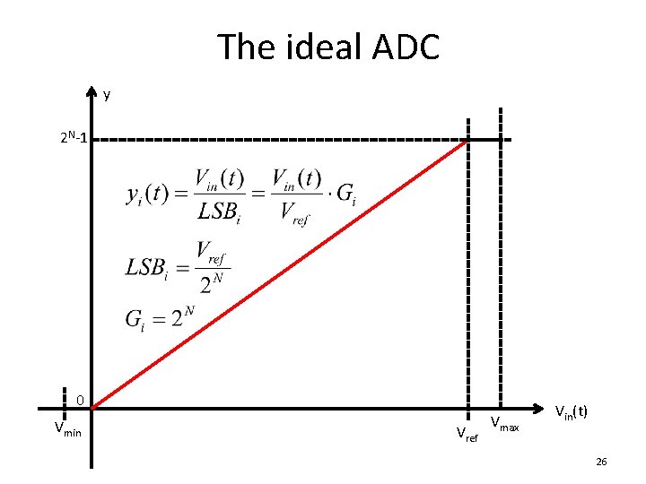
The ideal ADC y 2 N-1 0 Vmin Vref Vmax Vin(t) 26

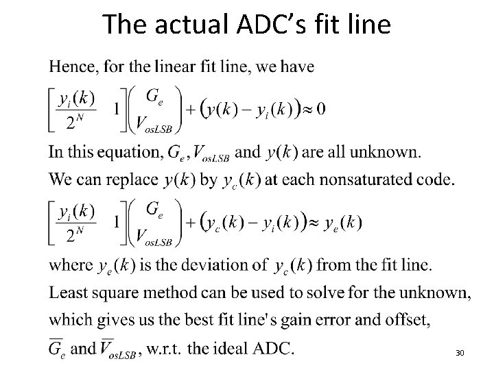
The actual ADC’s fit line DVFSR y 2 N-1 GE VFSR 0 Vmin Vros Vref Vmax Vin(t) 27

The actual ADC’s fit line 28

The actual ADC’s fit line 29

The actual ADC’s fit line 30

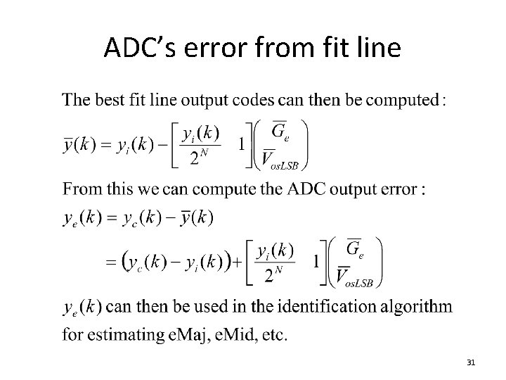
ADC’s error from fit line 31

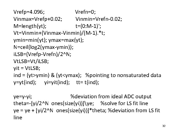
Vrefp=4. 096; Vrefn=0; Vinmax=Vrefp+0. 02; Vinmin=Vrefn-0. 02; M=length(yt); t=(0: M-1)'; Vt=Vinmin+(Vinmax-Vinmin)/(M-1). *t; ymin=min(yt); ymax=max(yt); N=ceil(log 2(ymax-ymin)); i. LSB=(Vrefp-Vrefn)/2^N; Vt. LSB=Vt/i. LSB; yit = Vt. LSB; ind = (yt>ymin) & (yt<ymax); %pointing to nonsaturated data y=yt(ind); yi=yit(ind); tt= t(ind); ye=y-yi; %deviation from ideal ADC output theta=-[yi/2^N ones(size(yi))]ye; %solve for LS fit line ye = ye + [yi/2^N ones(size(yi))]*theta; %deviation from LS fit line 32

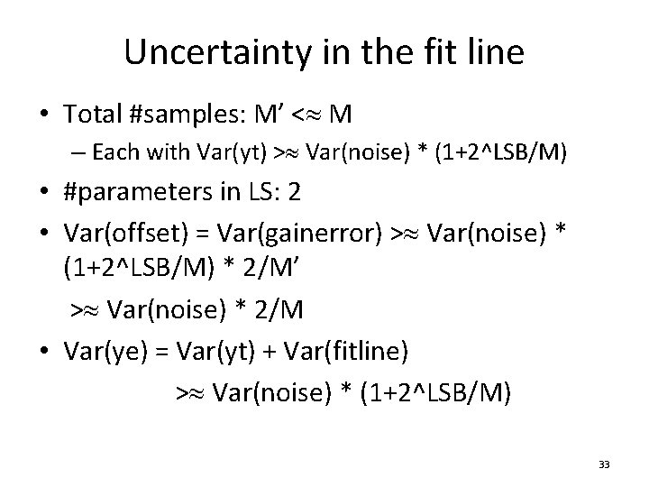
Uncertainty in the fit line • Total #samples: M’ < M – Each with Var(yt) > Var(noise) * (1+2^LSB/M) • #parameters in LS: 2 • Var(offset) = Var(gainerror) > Var(noise) * (1+2^LSB/M) * 2/M’ > Var(noise) * 2/M • Var(ye) = Var(yt) + Var(fitline) > Var(noise) * (1+2^LSB/M) 33

ADC output codes Example: 16 bit ADC, 2^14 samples Blue: yt Red: yit Sample time index 34

LS best fit line Ideal ADC output, real numbers LS best fit line offset real ADC output, integer numbers 35

LS best fit line offset + gainerror Idea ADC output, real numbers real ADC output, integer numbers, capped at 2^16 -1 36

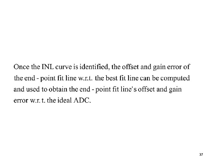
37

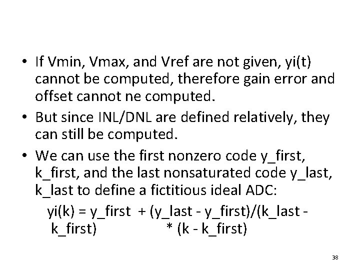
• If Vmin, Vmax, and Vref are not given, yi(t) cannot be computed, therefore gain error and offset cannot ne computed. • But since INL/DNL are defined relatively, they can still be computed. • We can use the first nonzero code y_first, k_first, and the last nonsaturated code y_last, k_last to define a fictitious ideal ADC: yi(k) = y_first + (y_last - y_first)/(k_last k_first) * (k - k_first) 38

Segmented nonparametric ID Expected Linear code Accurate source f(t) ADC C(t) + – + N. L error and noise + INL(C) n Code k: 0, 1, …, 2 -1 Segmented non parametric model for INL/DNL INL(k) ID goal: search for error terms that produce the best match at the observed output codes 39

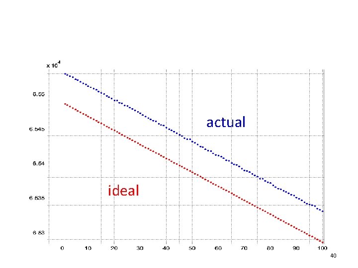
actual ideal 40

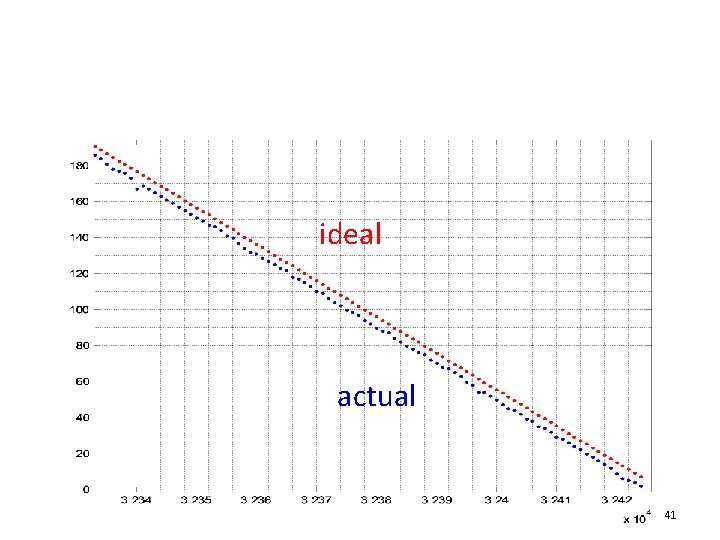
ideal actual 41

actual LS Fit Line 42

actual LS Fit Line 43

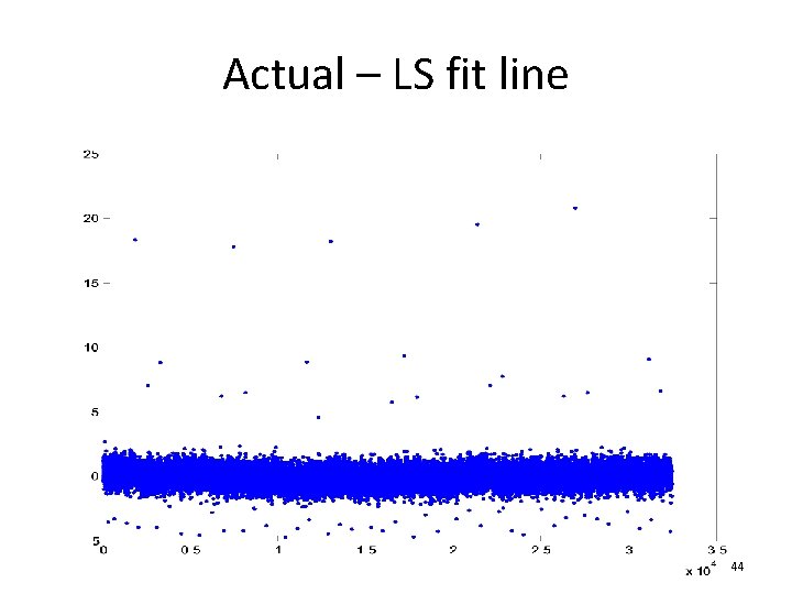
Actual – LS fit line 44

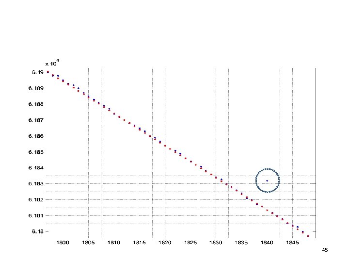
45

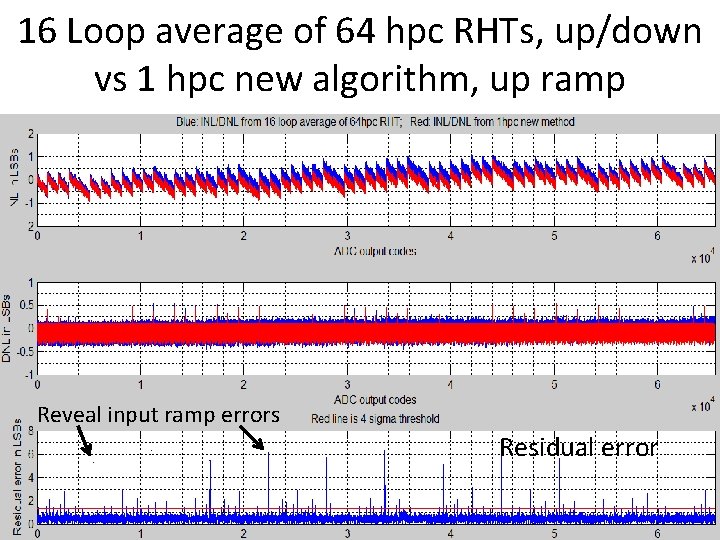
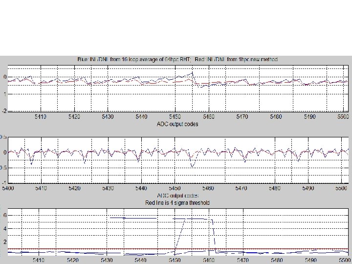
• There are quite a few excursion points / outliers / sparkles • Are they due to ADC errors? • Or are they due to input? • Histogram test totally misses all of them • New methods caught them 46

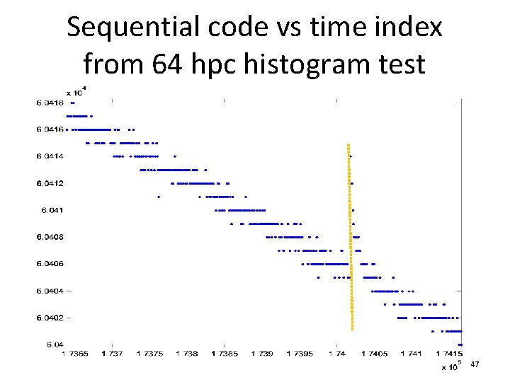
Sequential code vs time index from 64 hpc histogram test 47

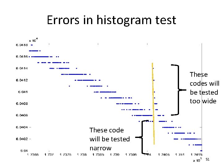
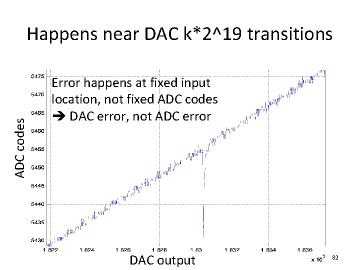
• Errors associated with specific horizontal locations are due to ADC • Errors associated with specific vertical locations are due to input • Since excursions crowds after vertical yellow line, errors are due to input: DAC error at a major carrier transition due to insufficient settling • ADC not bad 48

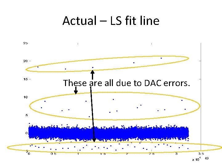
Actual – LS fit line These are all due to DAC errors. 49

• Once ADC output are tallied, all time domain information is lost. • Histogram masks existence of excursion points, sparkles, non-monotonic transfer curves, and so on. • The inclusion of DAC error induced excursion points causes RHT to be wrong at affected codes. • Increasing hpc or multi-loop averaging will not be able to remove such errors. • Such effects will be shown. 50

Errors in histogram test These codes will be tested too wide These code will be tested narrow 51

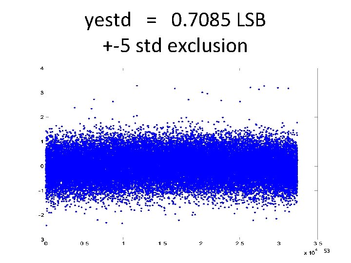
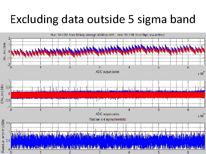
New algorithm immunity • New algorithm computes error from expected output (LS fit line, or sine wave fit) • If error var exceeds threshold, bad ADC or bad input, flag warning, stop processing • Else, use +- k * error standard deviation as threshold to exclude excursion points – Proper k depends on total number of point – For M = 1000’s, use k=4 – For M = 10, 000’s, use k = 5 – For M = 100, 000’s , use k = 6 • Total #valid samples becomes M” <= M’ < M 52

yestd = 0. 7085 LSB +-5 std exclusion 53

• If ADC is reasonably good and input is accurate, the number of points to be excluded will be very small if not 0 • Exclusion will have no effect on measurement accuracy or uncertainty 54

Segmented nonparametric ID Expected Linear code Accurate source f(t) ADC C(t) + – + N. L error and noise + INL(C) n Code k: 0, 1, …, 2 -1 Segmented non parametric model for INL/DNL INL(k) ID goal: search for error terms that produce the best match at the observed output codes 55

Segmented model identification • ye’s computed at all valid codes (nonsaturation, non-excursion) • ye’s contain ADC’s nonlinearity error and noise (including quantization) • They can be used as input to drive any identification algorithm to compute the unknowns: e. Maj(1 : 2^Maj), e. Mid(1 : 2^Mid), and e. Tail(1 : 2^Tail) 56

Segmented model identification • One possible way is to write one equation at each valid time instant k: e. Maj(M_k) + e. Mid(m_k) + e. Tail(T_k) ye_k where M_k, m_k, T_k are found based on the ADC output code yc_k at time k: M_k * 2^(N-Maj) + m_k * 2^Tail + T_k = yc_k • We have M” such eauations that are linear in the unknowns: e. Maj, e. Mid, and e. Tail • Can use LS to solve the unknowns 57

Segmented model identification • The LS solution minimizes the power of the residual errors • That may not be the “best” solution. • Plus, LS may be computationally intensive. • One may also minimize the L_ norm or the L_1 norm (power is L_2 norm squared) or a different norm • The “best” in the probability sense is the maximum likelihood solution. 58

A simple suboptimal solution • A 3 step solution • Each step uses sample means as solutions for parameters in that step • The most important part of the solution is optimal under certain assumption • Overall solution is computationally efficient, since it only requires picking samples and taking averages • Overall accuracy is decent as can be seen later 59

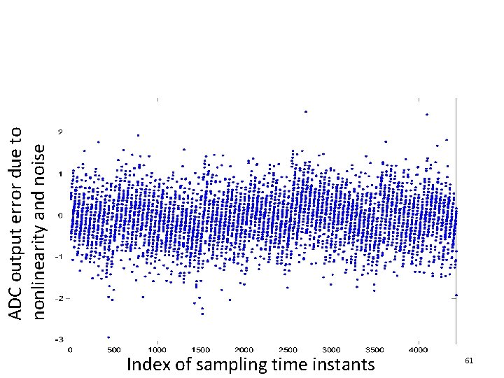
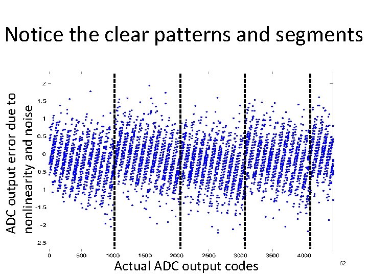
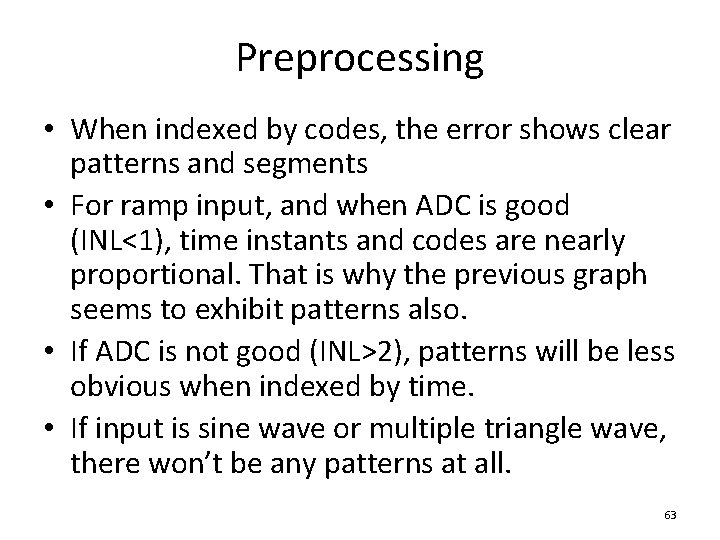
Preprocessing • The previous ye’s are sequentially index by the order of the sampling time instants • To be able to easily avoiding major carrier transitions, the ye’s are first sorted according to the output codes of the ADC • After this is done, the plot of ye’s will clearly show segments, as can be seen in the next two graphs 60

Index of sampling time instants 61 ADC output error due to nonlinearity and noise

ADC output error due to nonlinearity and noise Notice the clear patterns and segments Actual ADC output codes 62

Preprocessing • When indexed by codes, the error shows clear patterns and segments • For ramp input, and when ADC is good (INL<1), time instants and codes are nearly proportional. That is why the previous graph seems to exhibit patterns also. • If ADC is not good (INL>2), patterns will be less obvious when indexed by time. • If input is sine wave or multiple triangle wave, there won’t be any patterns at all. 63

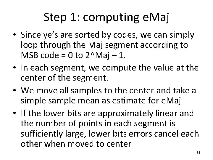
Step 1: computing e. Maj • Since ye’s are sorted by codes, we can simply loop through the Maj segment according to MSB code = 0 to 2^Maj – 1. • In each segment, we compute the value at the center of the segment. • We move all samples to the center and take a simple sample mean as estimate for e. Maj • If the lower bits are approximately linear and the number of points in each segment is sufficiently large, lower bits errors cancel each other when moved to center 64

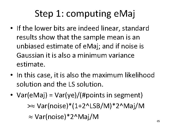
Step 1: computing e. Maj • If the lower bits are indeed linear, standard results show that the sample mean is an unbiased estimate of e. Maj; and if noise is Gaussian it is also a minimum variance estimate. • In this case, it is also the maximum likelihood solution and the LS solution. • Var(e. Maj) = Var(ye)/(#points in segment) > Var(noise)*(1+2^LSB/M)*2^Maj/M Var(noise)*2^Maj/M 65

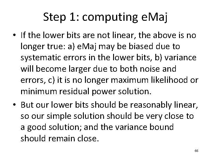
Step 1: computing e. Maj • If the lower bits are not linear, the above is no longer true: a) e. Maj may be biased due to systematic errors in the lower bits, b) variance will become larger due to both noise and errors, c) it is no longer maximum likelihood or minimum residual power solution. • But our lower bits should be reasonably linear, so our simple solution should be very close to a good solution; and the variance bound should remain close. 66

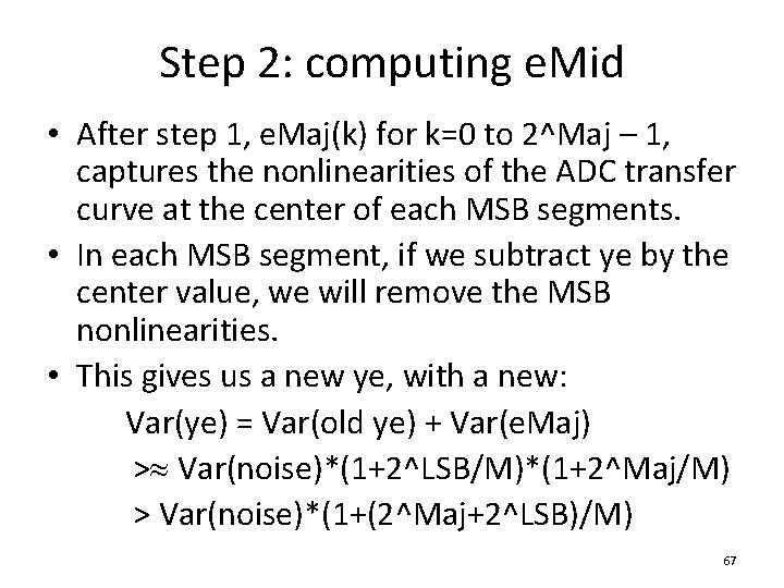
Step 2: computing e. Mid • After step 1, e. Maj(k) for k=0 to 2^Maj – 1, captures the nonlinearities of the ADC transfer curve at the center of each MSB segments. • In each MSB segment, if we subtract ye by the center value, we will remove the MSB nonlinearities. • This gives us a new ye, with a new: Var(ye) = Var(old ye) + Var(e. Maj) > Var(noise)*(1+2^LSB/M)*(1+2^Maj/M) > Var(noise)*(1+(2^Maj+2^LSB)/M) 67

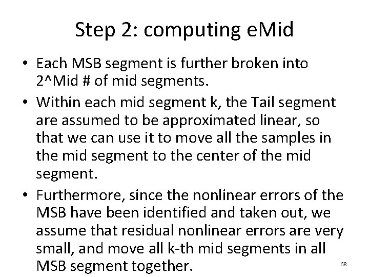
Step 2: computing e. Mid • Each MSB segment is further broken into 2^Mid # of mid segments. • Within each mid segment k, the Tail segment are assumed to be approximated linear, so that we can use it to move all the samples in the mid segment to the center of the mid segment. • Furthermore, since the nonlinear errors of the MSB have been identified and taken out, we assume that residual nonlinear errors are very small, and move all k-th mid segments in all MSB segment together. 68

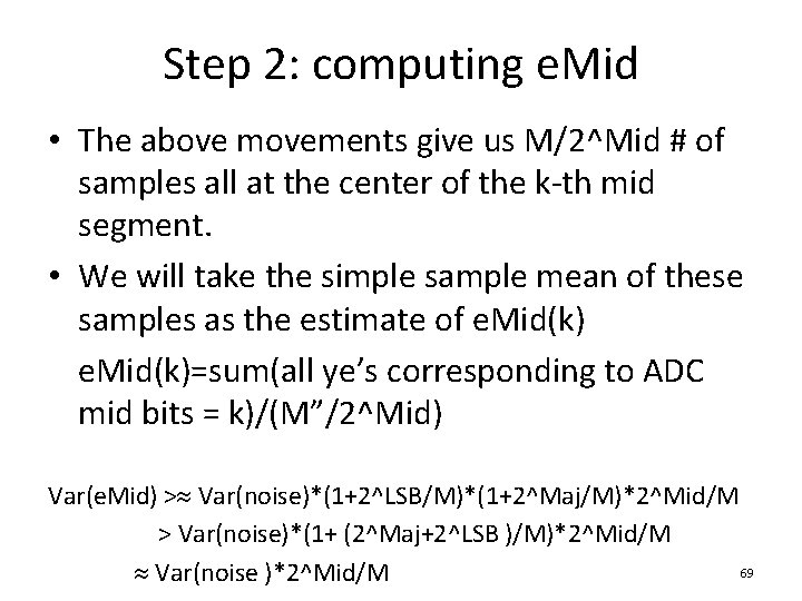
Step 2: computing e. Mid • The above movements give us M/2^Mid # of samples all at the center of the k-th mid segment. • We will take the simple sample mean of these samples as the estimate of e. Mid(k)=sum(all ye’s corresponding to ADC mid bits = k)/(M”/2^Mid) Var(e. Mid) > Var(noise)*(1+2^LSB/M)*(1+2^Maj/M)*2^Mid/M > Var(noise)*(1+ (2^Maj+2^LSB )/M)*2^Mid/M 69 Var(noise )*2^Mid/M

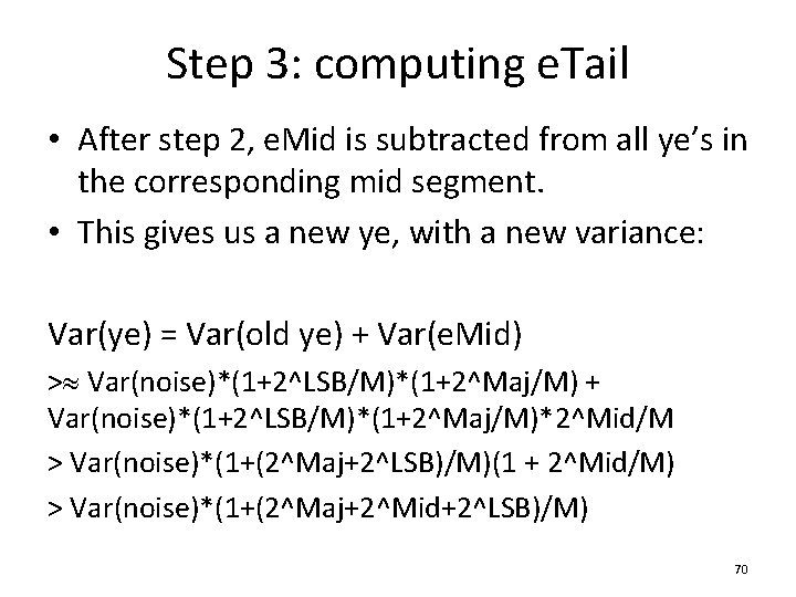
Step 3: computing e. Tail • After step 2, e. Mid is subtracted from all ye’s in the corresponding mid segment. • This gives us a new ye, with a new variance: Var(ye) = Var(old ye) + Var(e. Mid) > Var(noise)*(1+2^LSB/M)*(1+2^Maj/M) + Var(noise)*(1+2^LSB/M)*(1+2^Maj/M)*2^Mid/M > Var(noise)*(1+(2^Maj+2^LSB)/M)(1 + 2^Mid/M) > Var(noise)*(1+(2^Maj+2^Mid+2^LSB)/M) 70

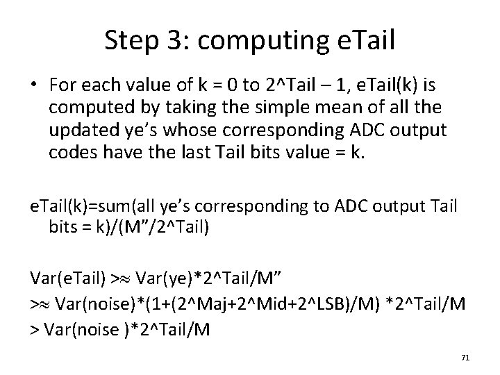
Step 3: computing e. Tail • For each value of k = 0 to 2^Tail – 1, e. Tail(k) is computed by taking the simple mean of all the updated ye’s whose corresponding ADC output codes have the last Tail bits value = k. e. Tail(k)=sum(all ye’s corresponding to ADC output Tail bits = k)/(M”/2^Tail) Var(e. Tail) > Var(ye)*2^Tail/M” > Var(noise)*(1+(2^Maj+2^Mid+2^LSB)/M) *2^Tail/M > Var(noise )*2^Tail/M 71

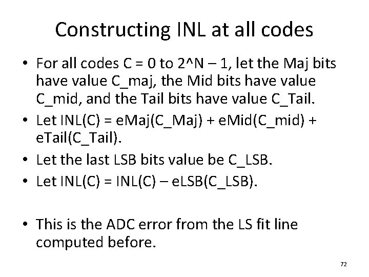
Constructing INL at all codes • For all codes C = 0 to 2^N – 1, let the Maj bits have value C_maj, the Mid bits have value C_mid, and the Tail bits have value C_Tail. • Let INL(C) = e. Maj(C_Maj) + e. Mid(C_mid) + e. Tail(C_Tail). • Let the last LSB bits value be C_LSB. • Let INL(C) = INL(C) – e. LSB(C_LSB). • This is the ADC error from the LS fit line computed before. 72

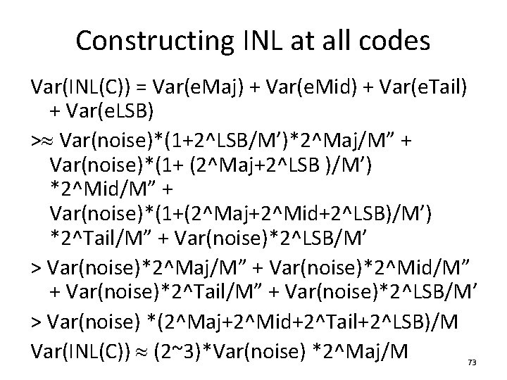
Constructing INL at all codes Var(INL(C)) = Var(e. Maj) + Var(e. Mid) + Var(e. Tail) + Var(e. LSB) > Var(noise)*(1+2^LSB/M’)*2^Maj/M” + Var(noise)*(1+ (2^Maj+2^LSB )/M’) *2^Mid/M” + Var(noise)*(1+(2^Maj+2^Mid+2^LSB)/M’) *2^Tail/M” + Var(noise)*2^LSB/M’ > Var(noise)*2^Maj/M” + Var(noise)*2^Mid/M” + Var(noise)*2^Tail/M” + Var(noise)*2^LSB/M’ > Var(noise) *(2^Maj+2^Mid+2^Tail+2^LSB)/M Var(INL(C)) (2~3)*Var(noise) *2^Maj/M 73

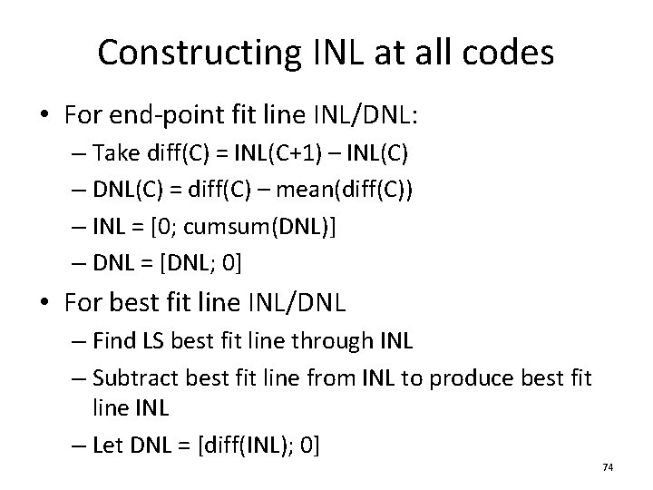
Constructing INL at all codes • For end-point fit line INL/DNL: – Take diff(C) = INL(C+1) – INL(C) – DNL(C) = diff(C) – mean(diff(C)) – INL = [0; cumsum(DNL)] – DNL = [DNL; 0] • For best fit line INL/DNL – Find LS best fit line through INL – Subtract best fit line from INL to produce best fit line INL – Let DNL = [diff(INL); 0] 74

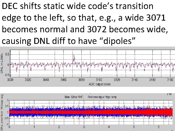
Wide/narrow code near Maj segment transitions • Whether wide/narrow code should belong to code after transition, or belong to code before transition, depends on architecture • For Capacitive SAR ADCs, a wide code happens after the transition; a narrow code or missing codes belong to before transition. • Use of on-chip DEC affects location of wide/narrow codes. • Decisions on wide/narrow code treatment need to be made with designers 75

Magnitude of ADC errors and residual errors after extracting INL/DNL • Magnitude of ADC errors can be used to detect – Sparkle codes, excursion samples – Settling problems in signal sources – Grossly poor converters • Magnitude of residual errors can be used to detect – Quality of INL/DNL results – Any trouble codes that require additional testing 76

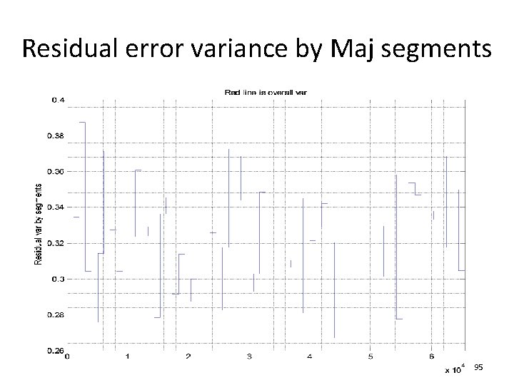
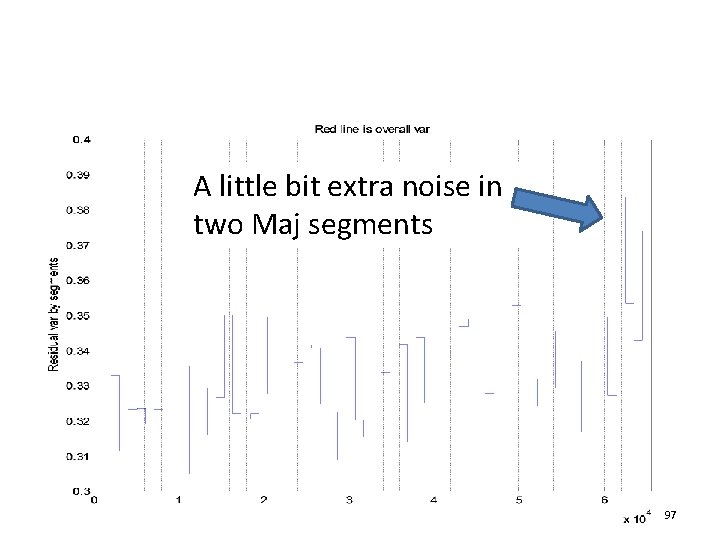
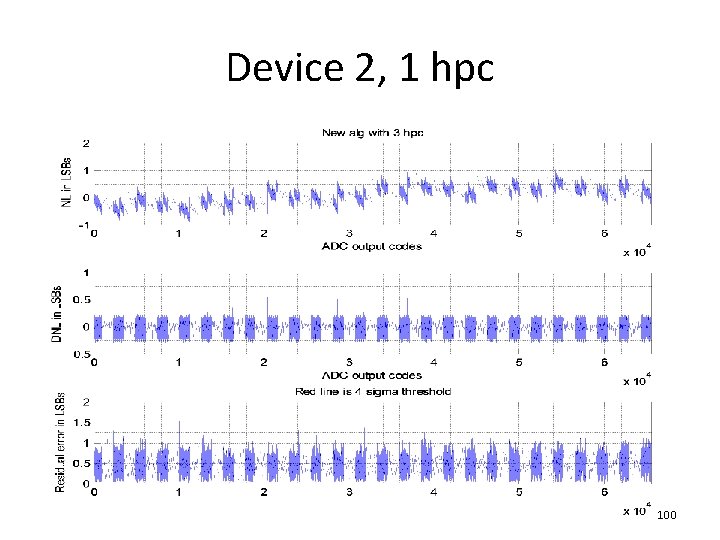
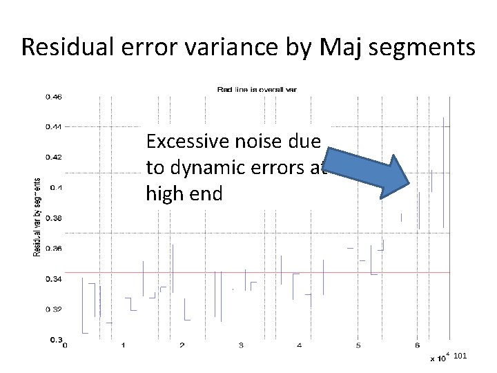
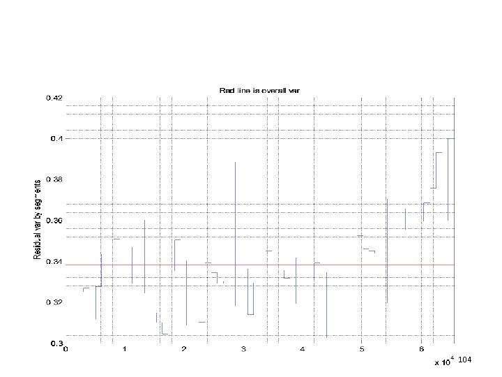
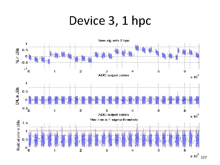
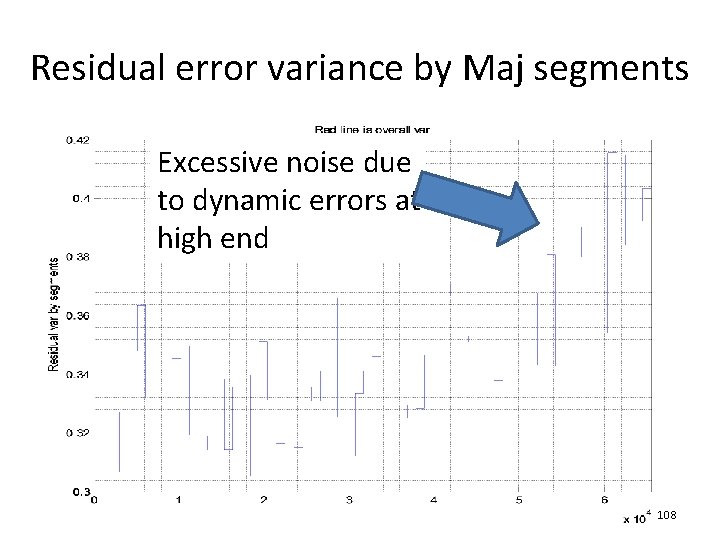
Variance of segment residual errors • Ideally the residual error should contain only noise effect • It should be wide in frequency, and should be about the same in all Maj segments • Due to dynamic errors, noise in various location can differ significantly • Variance of residual errors in each segment can be computed and compared to indicate the presence of significant dynamic errors • See device 2 and 3 for example. 77

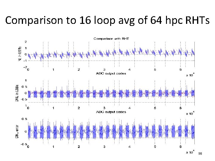
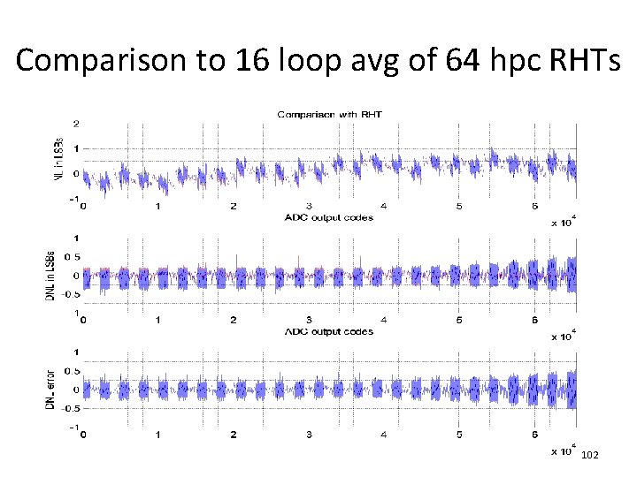
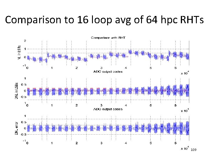
Measurement and comparison • Gayathri tested three different ADS 8332’s – 65 K point sine wave input output – 64 hits per code ramp input output • No servo loop results for reference • She tested each device with 64 hpc ramp histogram test, repeating 16 times • Average INL/DNL from 16 loops will be used as reference 78

Device 1 • We will show some intermediate results • This is to show the development process • And reveal certain problems with the tester • Final results are towards the end 79

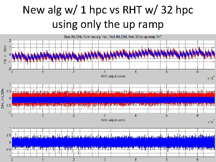
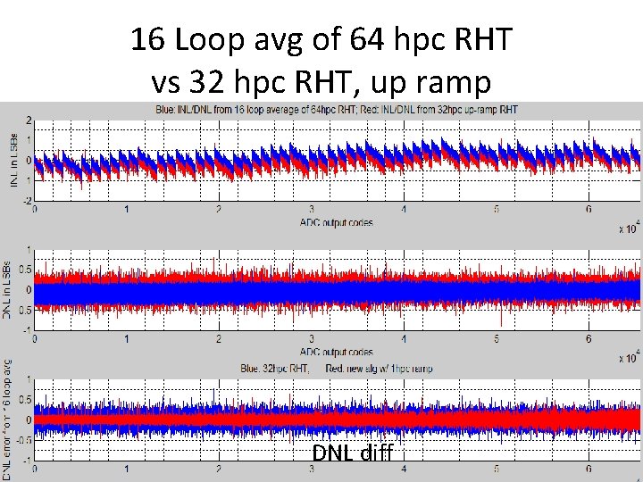
New alg w/ 1 hpc vs RHT w/ 32 hpc using only the up ramp 80

16 Loop average of 64 hpc RHTs, up/down vs 1 hpc new algorithm, up ramp Reveal input ramp errors Residual error 81

ADC codes Happens near DAC k*2^19 transitions Error happens at fixed input location, not fixed ADC codes DAC error, not ADC error DAC output 82

16 Loop avg of 64 hpc RHT vs 32 hpc RHT, up ramp DNL diff 83

Excluding data outside 5 sigma band 84

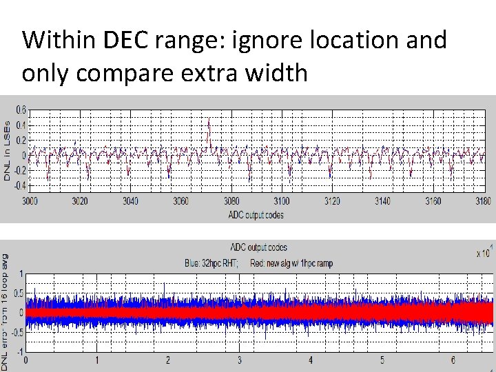
DEC shifts static wide code’s transition edge to the left, so that, e. g. , a wide 3071 becomes normal and 3072 becomes wide, causing DNL diff to have “dipoles” 85

Within DEC range: ignore location and only compare extra width 86

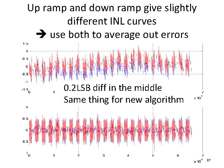
Up ramp and down ramp give slightly different INL curves use both to average out errors 0. 2 LSB diff in the middle Same thing for new algorithm 87

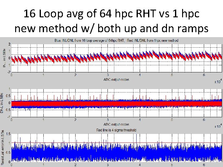
16 Loop avg of 64 hpc RHT vs 1 hpc new method w/ both up and dn ramps 88

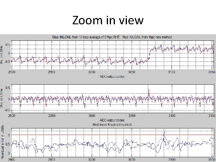
Zoom in view 89

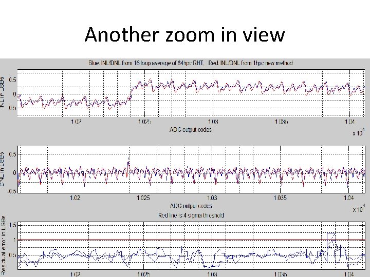
Another zoom in view 90

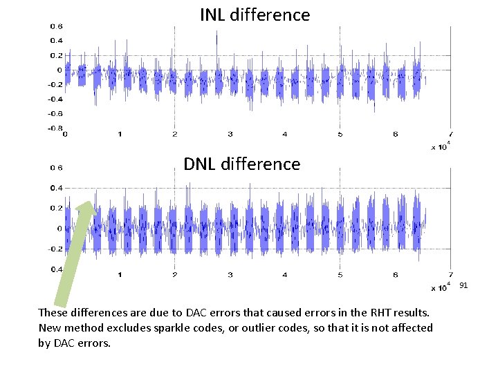
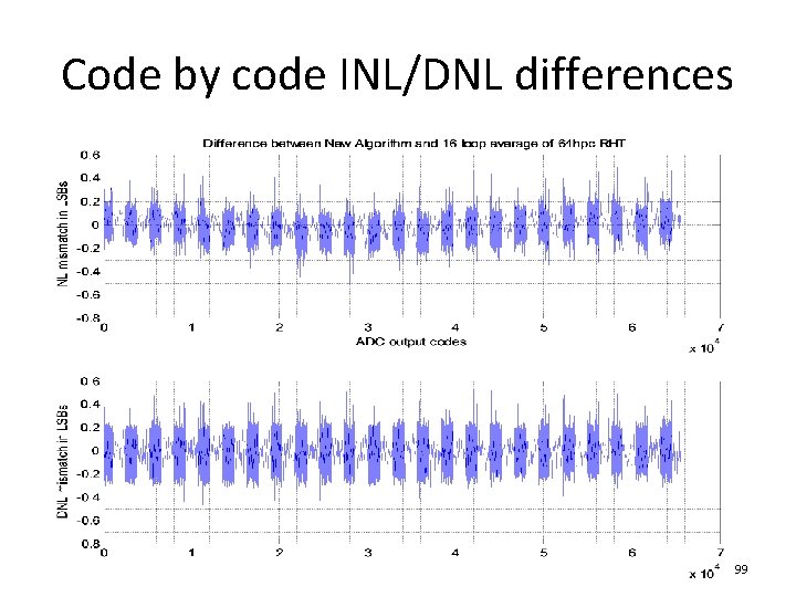
INL difference DNL difference 91 These differences are due to DAC errors that caused errors in the RHT results. New method excludes sparkle codes, or outlier codes, so that it is not affected by DAC errors.

92

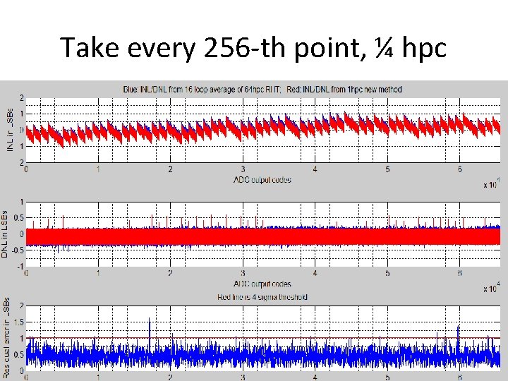
Take every 256 -th point, ¼ hpc 93

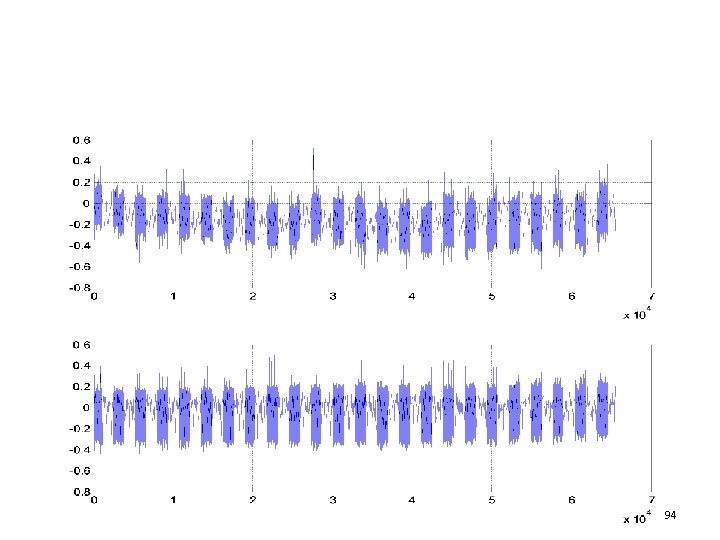
94

Residual error variance by Maj segments 95

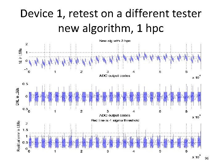
Device 1, retest on a different tester new algorithm, 1 hpc 96

A little bit extra noise in two Maj segments 97

Comparison to 16 loop avg of 64 hpc RHTs 98

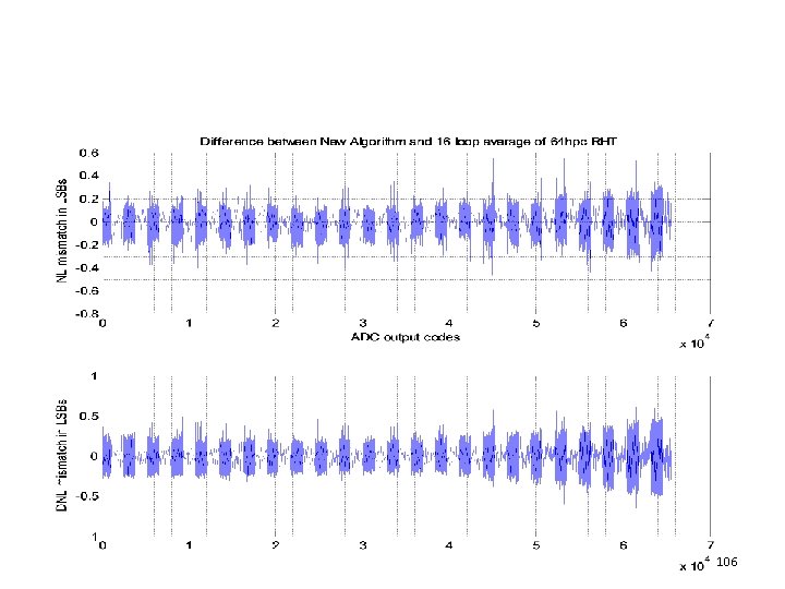
Code by code INL/DNL differences 99

Device 2, 1 hpc 100

Residual error variance by Maj segments Excessive noise due to dynamic errors at high end 101

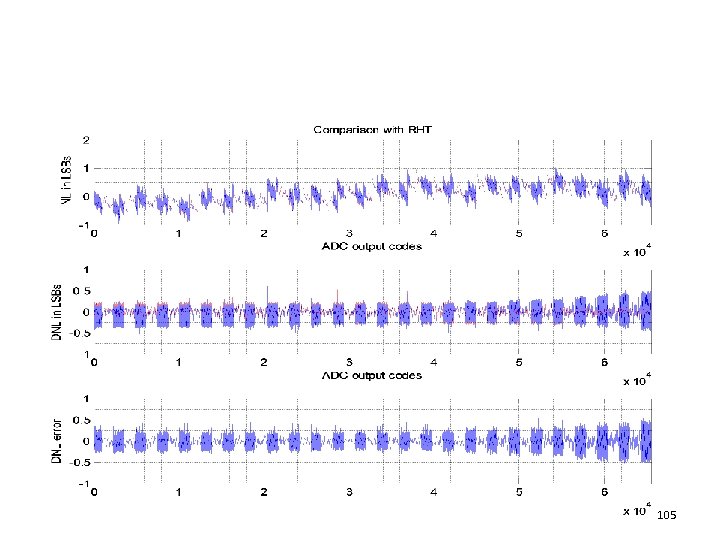
Comparison to 16 loop avg of 64 hpc RHTs 102

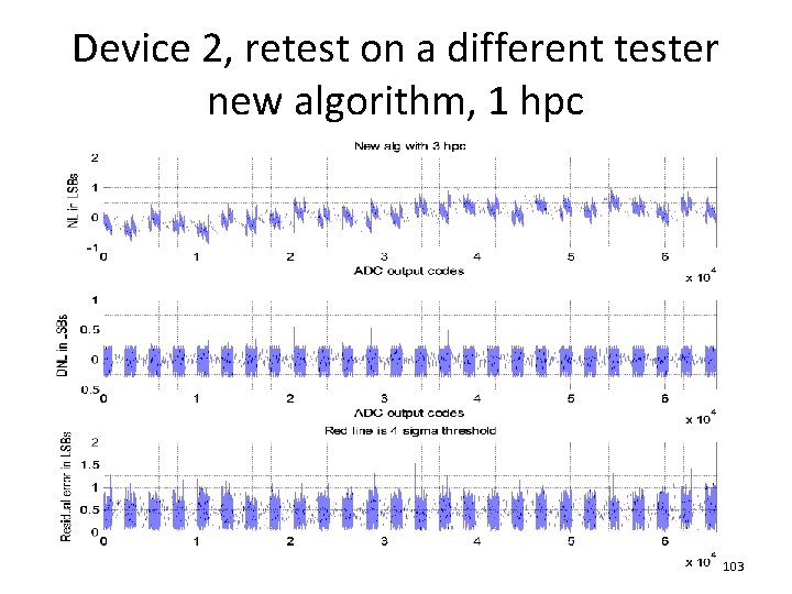
Device 2, retest on a different tester new algorithm, 1 hpc 103

104

105

106

Device 3, 1 hpc 107

Residual error variance by Maj segments Excessive noise due to dynamic errors at high end 108

Comparison to 16 loop avg of 64 hpc RHTs 109

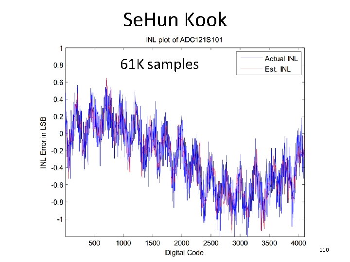
Se. Hun Kook 61 K samples 110