Inference for the mean vector Univariate Inference Let

Inference for the mean vector

Univariate Inference Let x 1, x 2, … , xn denote a sample of n from the normal distribution with mean m and variance s 2. Suppose we want to test H 0: m = m 0 vs HA : m ≠ m 0 The appropriate test is the t test: The test statistic: Reject H 0 if |t| > ta/2

The multivariate Test Let denote a sample of n from the p-variate normal distribution with mean vector and covariance matrix S. Suppose we want to test

Example For n = 10 students we measure scores on – Math proficiency test (x 1), – Science proficiency test (x 2), – English proficiency test (x 3) and – French proficiency test (x 4) The average score for each of the tests in previous years was 60. Has this changed?

The data

Summary Statistics the mean vector the sample covariance matrix

Roy’s Union- Intersection Principle This is a general procedure for developing a multivariate test from the corresponding univariate test. 1. Convert the multivariate problem to a univariate problem by considering an arbitrary linear combination of the observation vector.

2. 3. 4. 5. 6. Perform the test for the arbitrary linear combination of the observation vector. Repeat this for all possible choices of Reject the multivariate hypothesis if H 0 is rejected for any one of the choices for Accept the multivariate hypothesis if H 0 is accepted for all of the choices for Set the type I error rate for the individual tests so that the type I error rate for the multivariate test is a.

Application of Roy’s principle to the following situation Let denote a sample of n from the p-variate normal distribution with mean vector and covariance matrix S. Suppose we want to test Then u 1, …. un is a sample of n from the normal distribution with mean and variance.

to test we would use the test statistic:

and

Thus We will reject if

Using Roy’s Union- Intersection principle: We will reject We accept

i. e. We reject We accept

Consider the problem of finding: where

thus

Thus Roy’s Union- Intersection principle states: We reject We accept is called Hotelling’s T 2 statistic

Choosing the critical value for Hotelling’s T 2 statistic We reject , we need to find the sampling distribution of T 2 when H 0 is true. It turns out that if H 0 is true than has an F distribution with n 1 = p and n 2 = n - p

Thus Hotelling’s T 2 test We reject or if

Another derivation of Hotelling’s T 2 statistic Another method of developing statistical tests is the Likelihood ratio method. Suppose that the data vector, , has joint density Suppose that the parameter vector, , belongs to the set W. Let w denote a subset of W. Finally we want to test

The Likelihood ratio test rejects H 0 if

The situation Let denote a sample of n from the p-variate normal distribution with mean vector and covariance matrix S. Suppose we want to test

The Likelihood function is: and the Log-likelihood function is:

the Maximum Likelihood estimators of are and

the Maximum Likelihood estimators of when H 0 is true are: and

The Likelihood function is: now

Thus similarly

and

Note: Let

and Now and

Also

Thus

Thus using

Then Thus to reject H 0 if l < la This is the same as Hotelling’s T 2 test if

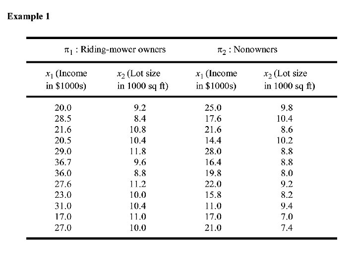
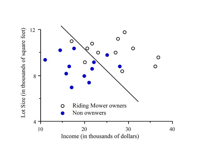
Example For n = 10 students we measure scores on – Math proficiency test (x 1), – Science proficiency test (x 2), – English proficiency test (x 3) and – French proficiency test (x 4) The average score for each of the tests in previous years was 60. Has this changed?

The data

Summary Statistics

Inference for the mean vector

Univariate Inference Let x 1, x 2, … , xn denote a sample of n from the normal distribution with mean m and variance s 2. Suppose we want to test H 0: m = m 0 vs HA : m ≠ m 0 The appropriate test is the t test: The test statistic: Reject H 0 if |t| > ta/2

Hotelling’s T 2 statistic and test We reject

Example For n = 10 students we measure scores on – Math proficiency test (x 1), – Science proficiency test (x 2), – English proficiency test (x 3) and – French proficiency test (x 4) The average score for each of the tests in previous years was 60. Has this changed?

The data

Summary Statistics

The two sample problem

Univariate Inference Let x 1, x 2, … , xn denote a sample of n from the normal distribution with mean mx and variance s 2. Let y 1, y 2, … , ym denote a sample of n from the normal distribution with mean my and variance s 2. Suppose we want to test H 0: mx = my vs HA : mx ≠ my

The appropriate test is the t test: The test statistic: Reject H 0 if |t| > ta/2 d. f. = n + m -2

The multivariate Test Let denote a sample of n from the p-variate normal distribution with mean vector and covariance matrix S. Let denote a sample of m from the p-variate normal distribution with mean vector and covariance matrix S. Suppose we want to test

Hotelling’s T 2 statistic for the two sample problem if H 0 is true than has an F distribution with n 1 = p and n 2 = n +m – p - 1

Thus Hotelling’s T 2 test We reject

Example 2 Annual financial data are collected for firms approximately 2 years prior to bankruptcy and for financially sound firms at about the same point in time. The data on the four variables • x 1 = CF/TD = (cash flow)/(total debt), • x 2 = NI/TA = (net income)/(Total assets), • x 3 = CA/CL = (current assets)/(current liabilties, and • x 4 = CA/NS = (current assets)/(net sales) are given in the following table.

The data are given in the following table:

Hotelling’s T 2 test A graphical explanation

Hotelling’s T 2 statistic for the two sample problem

is the test statistic for testing:

Hotelling’s T 2 test X 2 Popn A Popn B X 1

X 2 Univariate test for X 1 Popn A Popn B X 1

X 2 Univariate test for X 2 Popn A Popn B X 1

X 2 Univariate test for a 1 X 1 + a 2 X 2 Popn A Popn B X 1

Mahalanobis distance A graphical explanation

Euclidean distance

Mahalanobis distance: S, a covariance matrix

Hotelling’s T 2 statistic for the two sample problem

Case I X 2 Popn A Popn B X 1

Case II X 2 Popn A Popn B X 1

In Case I the Mahalanobis distance between the mean vectors is larger than in Case II, even though the Euclidean distance is smaller. In Case I there is more separation between the two bivariate normal distributions

Discrimination and Classification

Discrimination Situation: We have two or more populations p 1, p 2, etc (possibly p-variate normal). The populations are known (or we have data from each population) We have data for a new case (population unknown) and we want to identify the which population for which the new case is a member.

Examples

The Basic Problem Suppose that the data from a new case x 1, … , xp has joint density function either : p 1: f(x 1, … , xn) or p 2: g(x 1, … , xn) We want to make the decision to D 1: Classify the case in p 1 (f is the correct distribution) or D 2: Classify the case in p 2 (g is the correct distribution)

The Two Types of Errors 1. Misclassifying the case in p 1 when it actually lies in p 2. Let P[1|2] = P[D 1|p 2] = probability of this type of error 2. Misclassifying the case in p 2 when it actually lies in p 1. Let P[2|1] = P[D 2|p 1] = probability of this type of error This is similar Type I and Type II errors in hypothesis testing.

Note: A discrimination scheme is defined by splitting p – dimensional space into two regions. 1. C 1 = the region were we make the decision D 1. (the decision to classify the case in p 1) 2. C 2 = the region were we make the decision D 2. (the decision to classify the case in p 2)

There can be several approaches to determining the regions C 1 and C 2. All concerned with taking into account the probabilities of misclassification P[2|1] and P[1|2] 1. Set up the regions C 1 and C 2 so that one of the probabilities of misclassification , P[2|1] say, is at some low acceptable value a. Accept the level of the other probability of misclassification P[1|2] = b.

2. Set up the regions C 1 and C 2 so that the total probability of misclassification: P[Misclassification] = P[1] P[2|1] + P[2]P[1|2] is minimized P[1] = P[the case belongs to p 1] P[2] = P[the case belongs to p 2]

3. Set up the regions C 1 and C 2 so that the total expected cost of misclassification: E[Cost of Misclassification] = c 2|1 P[1] P[2|1] + c 1|2 P[2]P[1|2] is minimized P[1] = P[the case belongs to p 1] P[2] = P[the case belongs to p 2] c 2|1= the cost of misclassifying the case in p 2 when the case belongs to p 1. c 1|2= the cost of misclassifying the case in p 1 when the case belongs to p 2.

4. Set up the regions C 1 and C 2 The two types of error are equal: P[2|1] = P[1|2]

Computer security: p 1: Valid users p 2: Imposters P[2|1] = P[identifying a valid user as an imposter] P[1|2] = P[identifying an imposter as a valid user ] P[1] = P[valid user] P[2] = P[imposter] c 2|1= the cost of identifying the user as an imposter when the user is a valid user. c 1|2= the cost of identifying the user as a valid user when the user is an imposter.

This problem can be viewed as an Hypothesis testing problem H 0: p 1 is the correct population HA: p 2 is the correct population P[2|1] = a P[1|2] = b Power = 1 - b

The Neymann-Pearson Lemma Suppose that the data x 1, … , xn has joint density function f(x 1, … , xn ; q) where q is either q 1 or q 2. Let g(x 1, … , xn) = f(x 1, … , xn ; q 1) and h(x 1, … , xn) = f(x 1, … , xn ; q 2) We want to test H 0: q = q 1 (g is the correct distribution) against HA: q = q 2 (h is the correct distribution)

The Neymann-Pearson Lemma states that the Uniformly Most Powerful (UMP) test of size a is to reject H 0 if: and accept H 0 if: where ka is chosen so that the test is of size a.

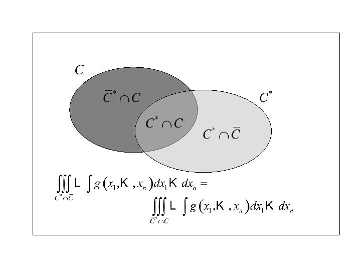
Proof: Let C be the critical region of any test of size We want to show that Note: a. Let

hence and Thus

and

Thus and when we add the common quantity Q. E. D. to both sides.

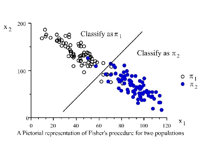
Fishers Linear Discriminant Function. Suppose that x 1, … , xp is either data from a p-variate Normal distribution with mean vector: The covariance matrix S is the same for both populations p 1 and p 2.

The Neymann-Pearson Lemma states that we should classify into populations p 1 and p 2 using: That is make the decision D 1 : population is p 1 if l ≥ ka

or or and Finally we make the decision D 1 : population is p 1 if where

The function Is called Fisher’s linear discriminant function

In the case where the populations are unknown but estimated from data Fisher’s linear discriminant function

Example 2 Annual financial data are collected for firms approximately 2 years prior to bankruptcy and for financially sound firms at about the same point in time. The data on the four variables • x 1 = CF/TD = (cash flow)/(total debt), • x 2 = NI/TA = (net income)/(Total assets), • x 3 = CA/CL = (current assets)/(current liabilties, and • x 4 = CA/NS = (current assets)/(net sales) are given in the following table.

The data are given in the following table: