Approximate Gaussian Elimination for Laplacians Speaker Rasmus Kyng

Approximate Gaussian Elimination for Laplacians Speaker Rasmus Kyng Harvard University Joint work with Sushant Sachdeva UToronto 11/27/2018

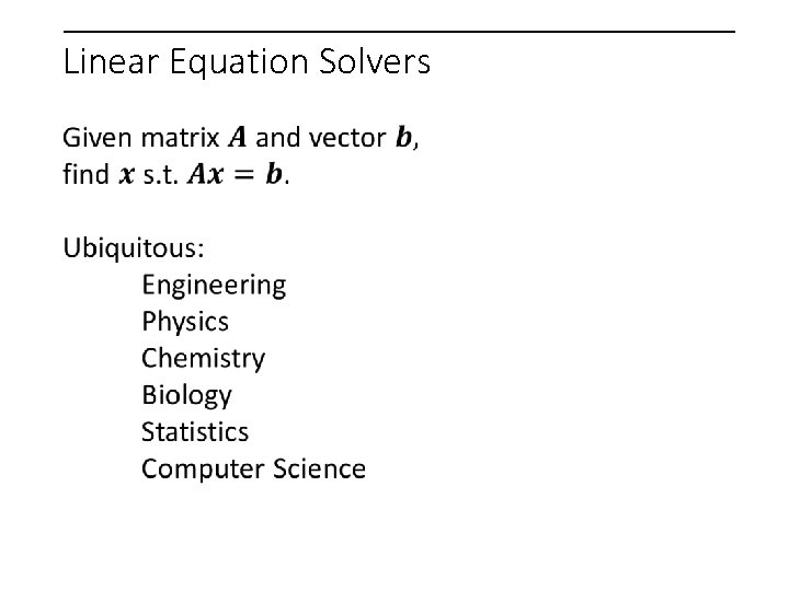
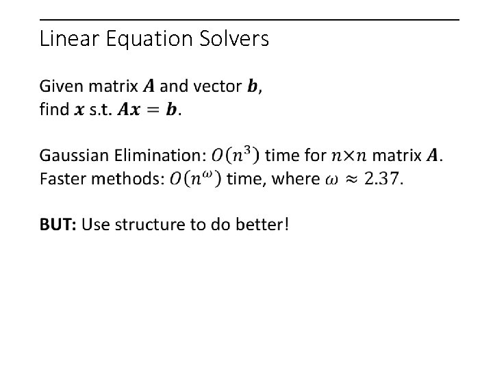
Linear Equation Solvers

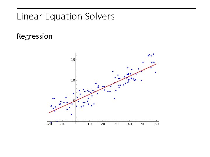
Linear Equation Solvers Regression

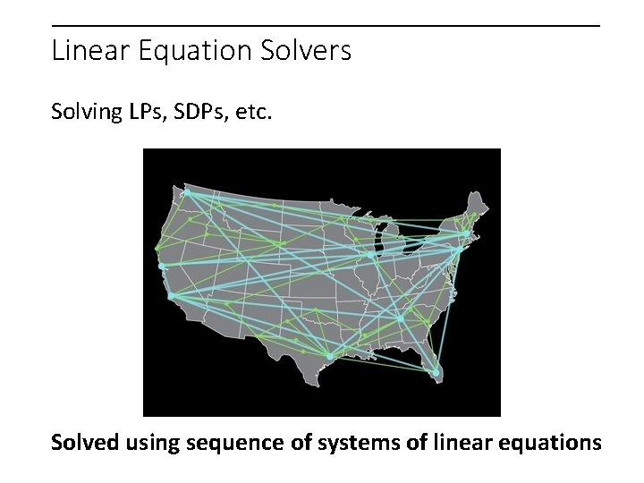
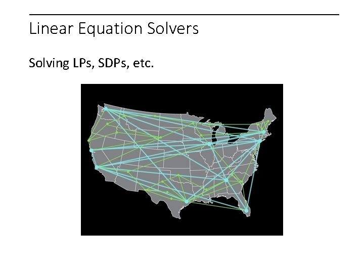
Linear Equation Solvers Solving LPs, SDPs, etc. Solved using sequence of systems of linear equations

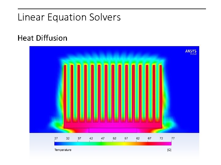
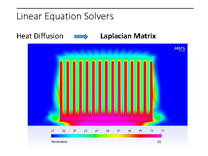
Linear Equation Solvers Heat Diffusion

Linear Equation Solvers

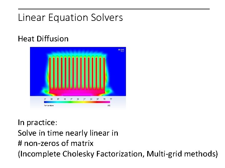
Linear Equation Solvers Heat Diffusion In practice: Solve in time nearly linear in # non-zeros of matrix (Incomplete Cholesky Factorization, Multi-grid methods)

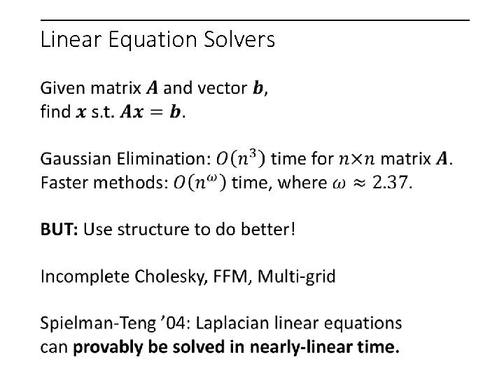
Linear Equation Solvers

Linear Equation Solvers Heat Diffusion Laplacian Matrix

Linear Equation Solvers Solving LPs, SDPs, etc.

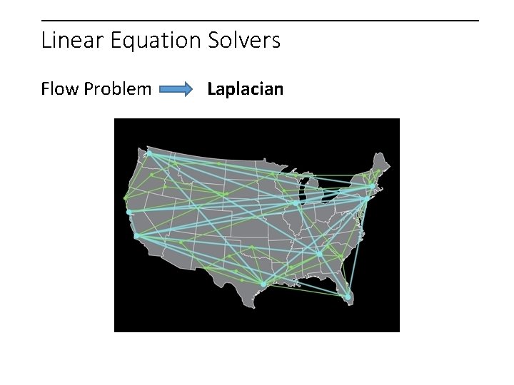
Linear Equation Solvers Flow Problem Laplacian

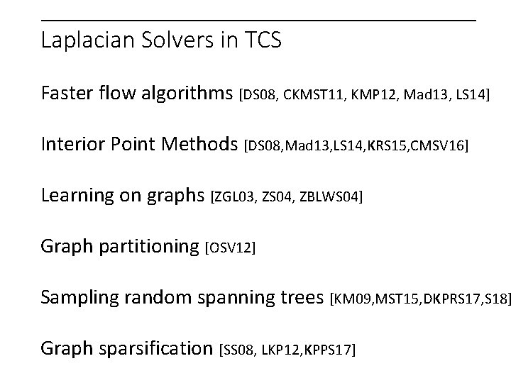
Laplacian Solvers in TCS Faster flow algorithms [DS 08, CKMST 11, KMP 12, Mad 13, LS 14] Interior Point Methods [DS 08, Mad 13, LS 14, KRS 15, CMSV 16] Learning on graphs [ZGL 03, ZS 04, ZBLWS 04] Graph partitioning [OSV 12] Sampling random spanning trees [KM 09, MST 15, DKPRS 17, S 18] Graph sparsification [SS 08, LKP 12, KPPS 17]

Laplacian Solvers in TCS Many papers improving the Laplacian Solver: [KMP 10, KMP 11, KOSZ 13, LS 13, CKM+14, PS 14, LPS 16] Simpler, faster, parallelizable

Beyond Laplacian Solvers Symmetric Diagonally Dominant [G 96] Planar 2 D Truss Stiffness Matrices [DS 07] Simplicial 3 D Truss Stiffness Matrices [KPSZ 18] Symmetric M-matrices [DS 08] Connection Laplacians and BDD matrices [KLPSS 16] Directed Laplacians [CKPPSV 16, CKPPRSV 16, CKKPPRS 18] Hardness for many other classes [KZ 17]

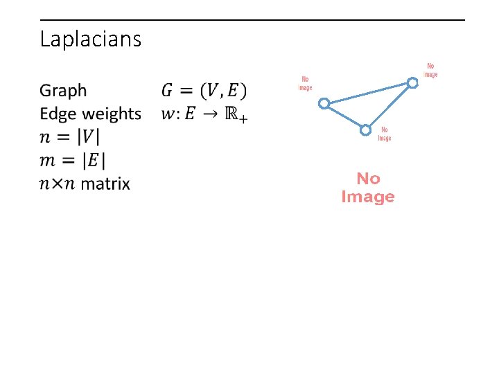
Laplacians

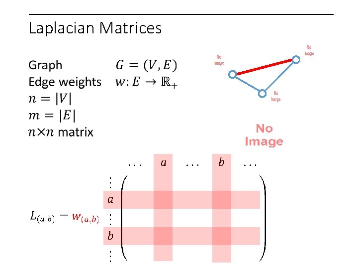
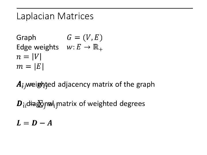
Laplacian Matrices

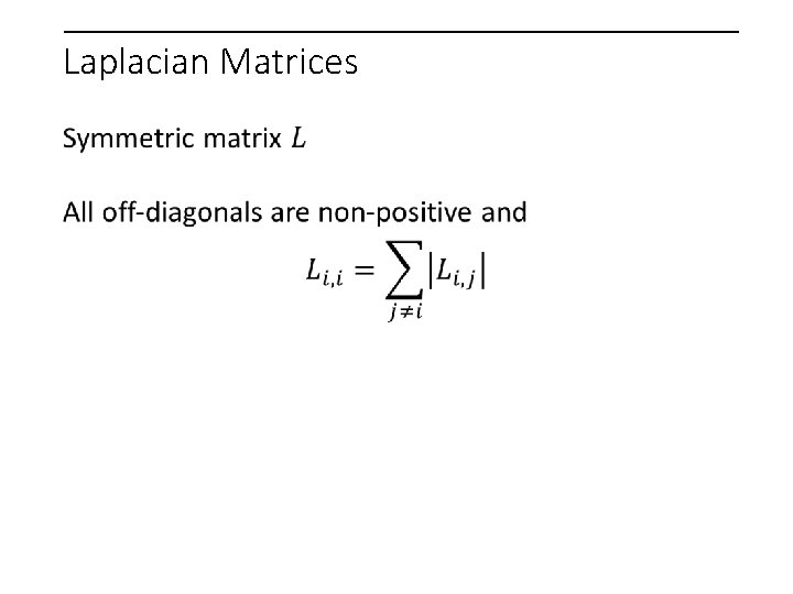
Laplacian Matrices

Laplacian Matrices

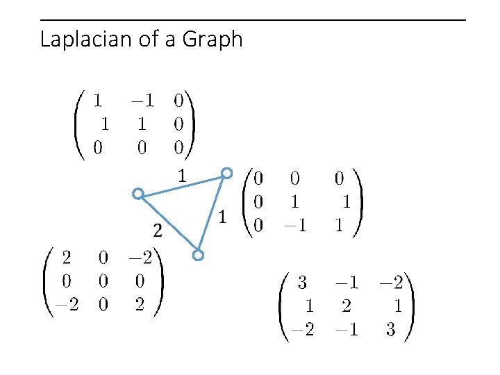
Laplacian of a Graph

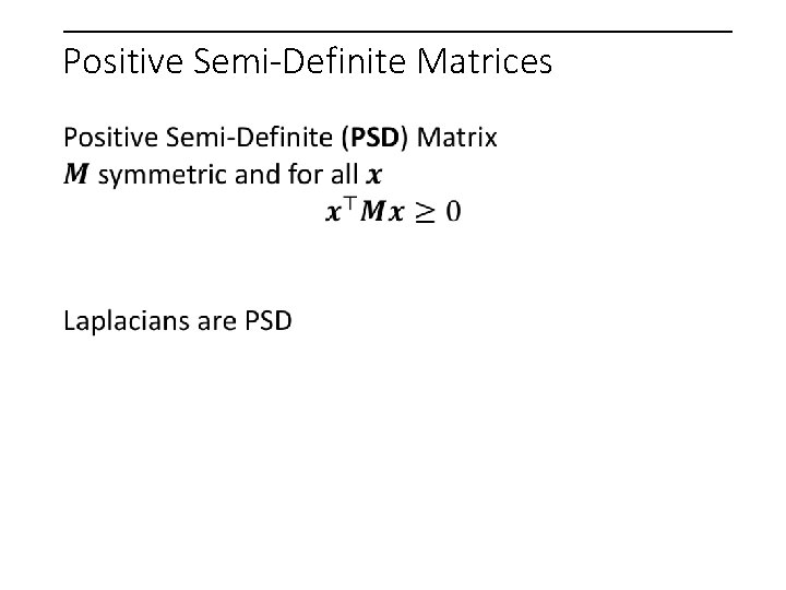
Positive Semi-Definite Matrices

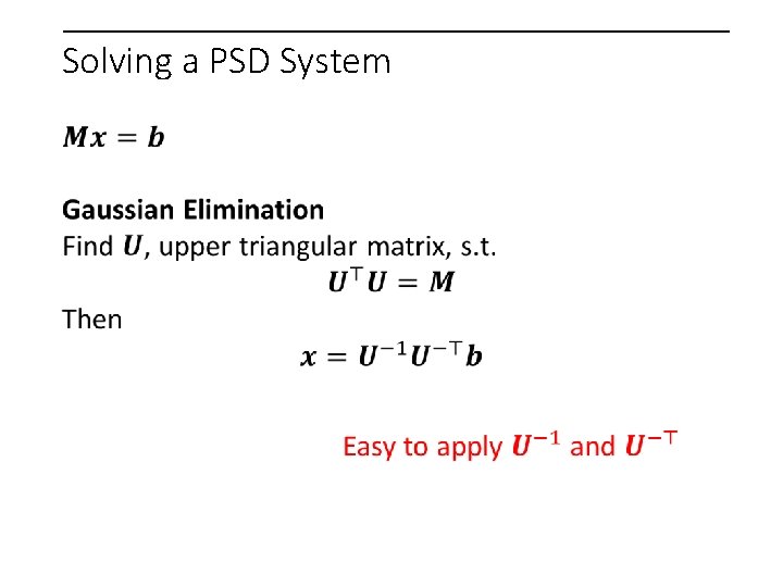
Solving a PSD System

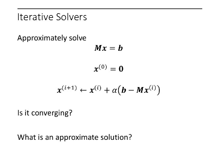
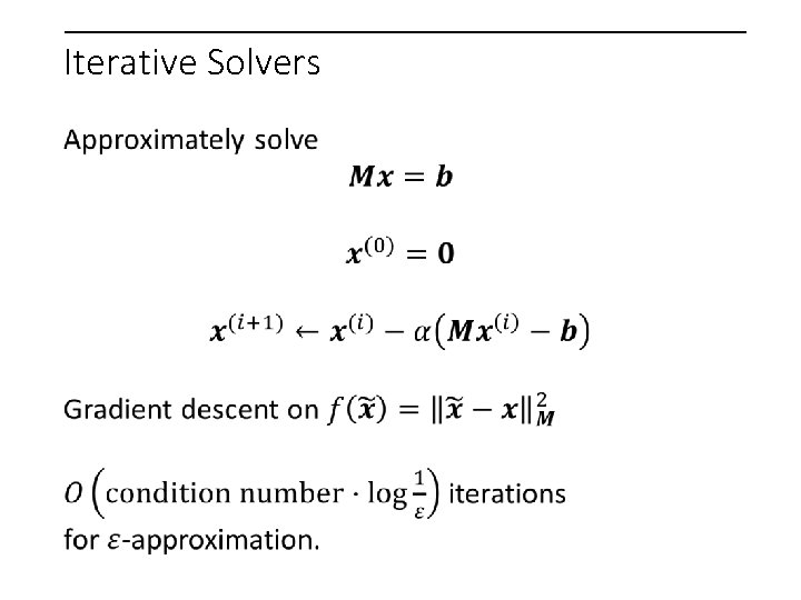
Iterative Solvers

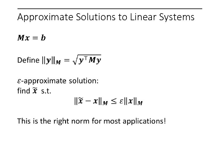
Approximate Solutions to Linear Systems

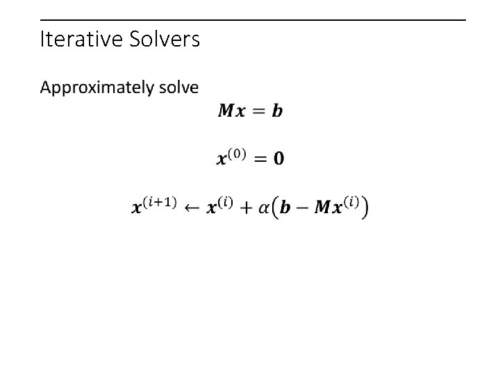
Iterative Solvers

Iterative Solvers

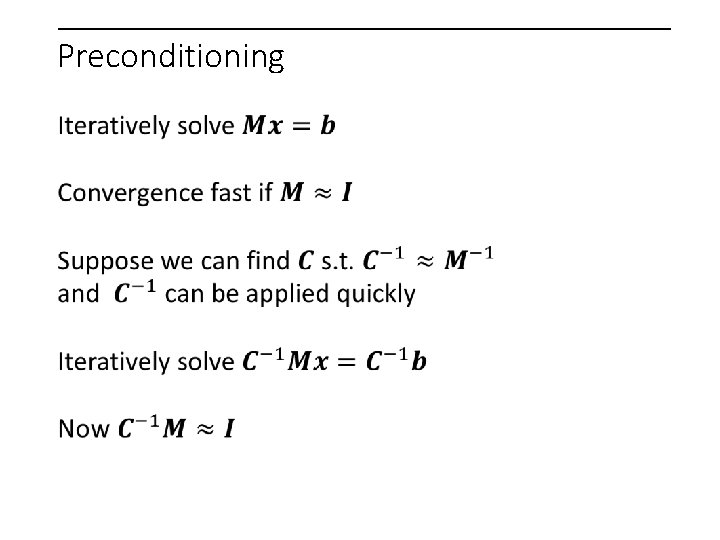
Preconditioning

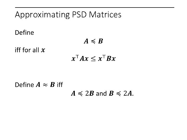
Approximating PSD Matrices

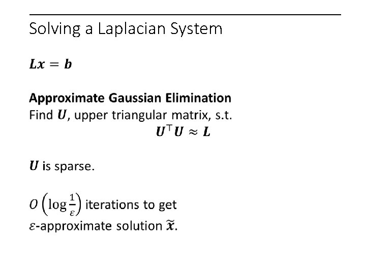
Solving a Laplacian System

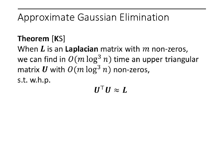
Approximate Gaussian Elimination

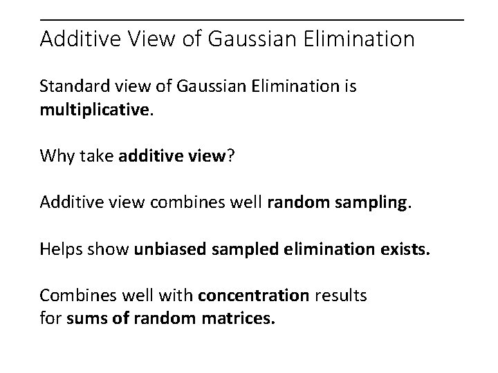
Additive View of Gaussian Elimination Standard view of Gaussian Elimination is multiplicative. Why take additive view? Additive view combines well random sampling. Helps show unbiased sampled elimination exists. Combines well with concentration results for sums of random matrices.

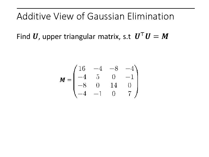
Additive View of Gaussian Elimination

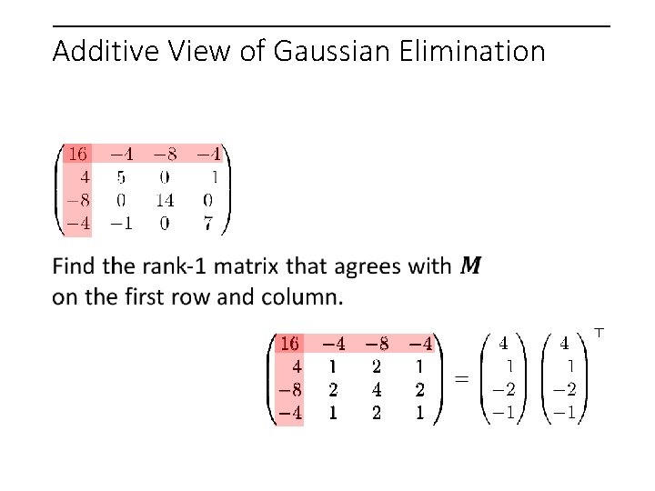
Additive View of Gaussian Elimination

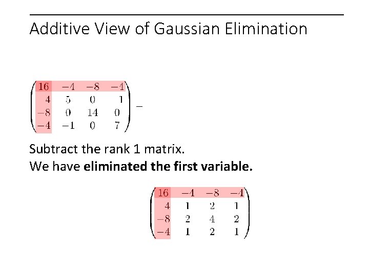
Additive View of Gaussian Elimination Subtract the rank 1 matrix. We have eliminated the first variable.

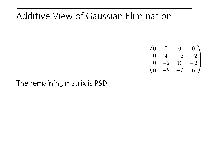
Additive View of Gaussian Elimination The remaining matrix is PSD.

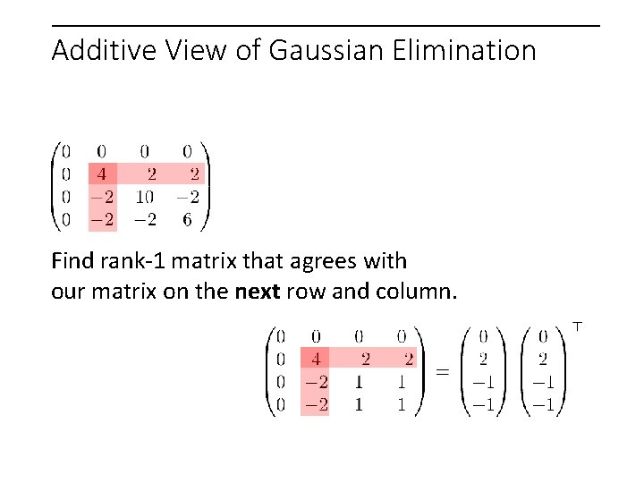
Additive View of Gaussian Elimination Find rank-1 matrix that agrees with our matrix on the next row and column.

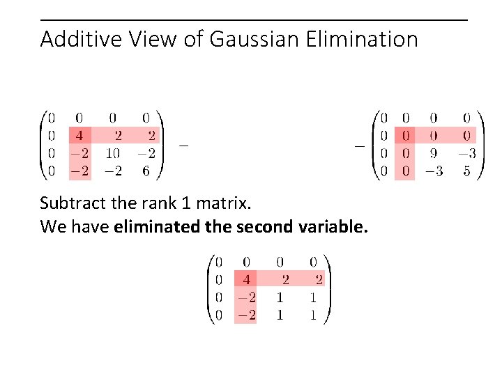
Additive View of Gaussian Elimination Subtract the rank 1 matrix. We have eliminated the second variable.

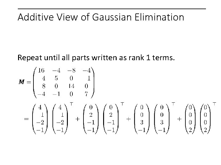
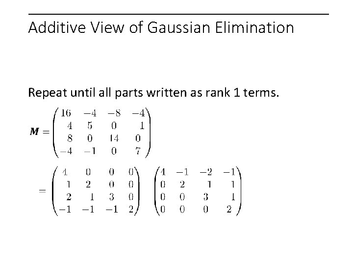
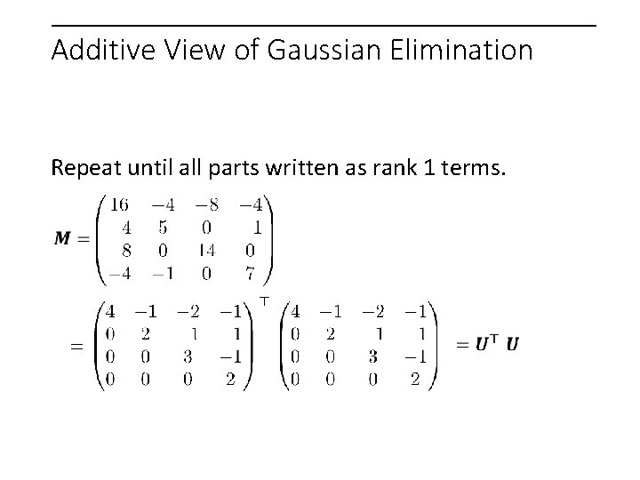
Additive View of Gaussian Elimination Repeat until all parts written as rank 1 terms.

Additive View of Gaussian Elimination Repeat until all parts written as rank 1 terms.

Additive View of Gaussian Elimination Repeat until all parts written as rank 1 terms.

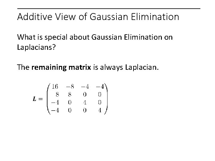
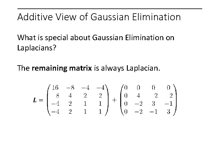
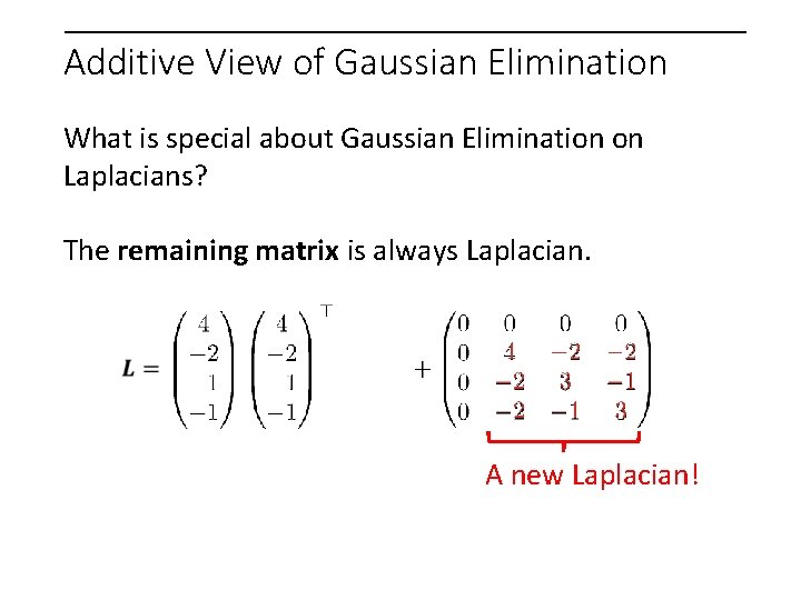
Additive View of Gaussian Elimination What is special about Gaussian Elimination on Laplacians? The remaining matrix is always Laplacian.

Additive View of Gaussian Elimination What is special about Gaussian Elimination on Laplacians? The remaining matrix is always Laplacian.

Additive View of Gaussian Elimination What is special about Gaussian Elimination on Laplacians? The remaining matrix is always Laplacian. A new Laplacian!

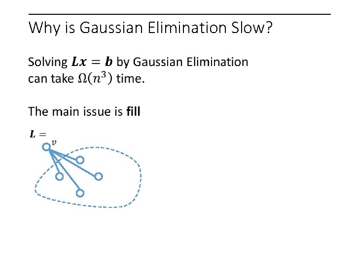
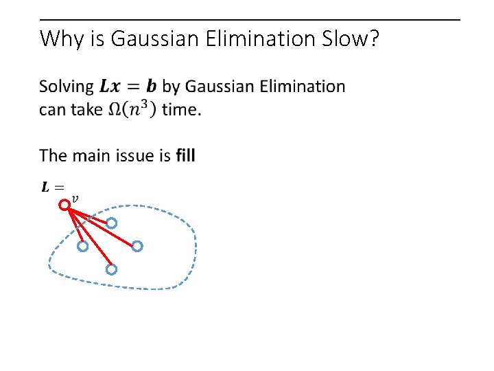
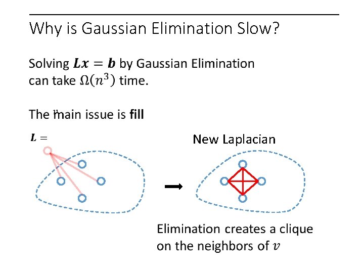
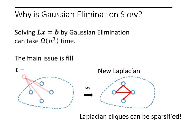
Why is Gaussian Elimination Slow?

Why is Gaussian Elimination Slow?

Why is Gaussian Elimination Slow? New Laplacian

Why is Gaussian Elimination Slow? New Laplacian cliques can be sparsified!

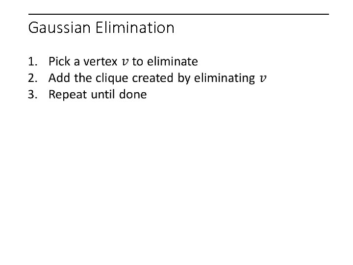
Gaussian Elimination

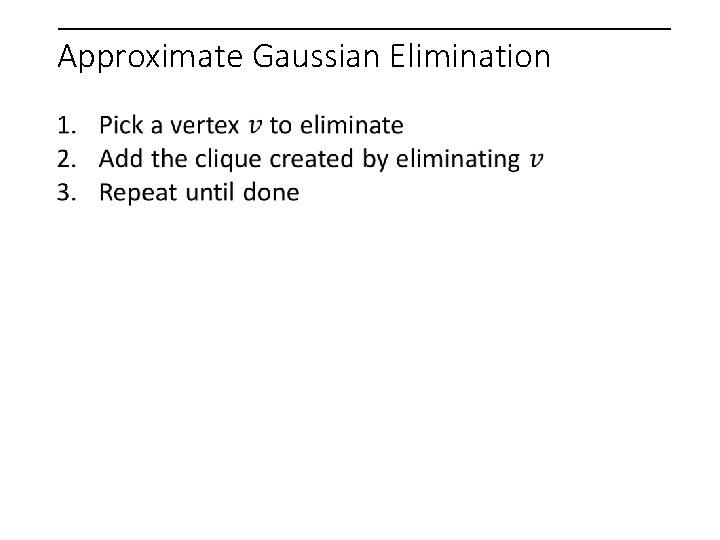
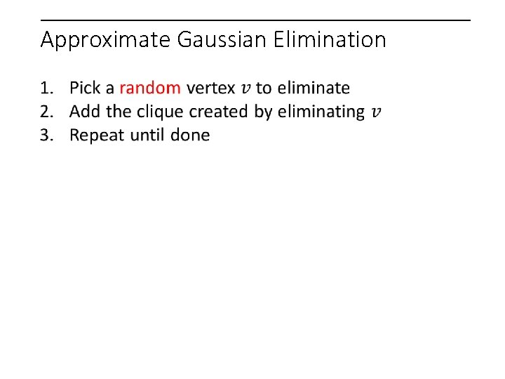
Approximate Gaussian Elimination

Approximate Gaussian Elimination

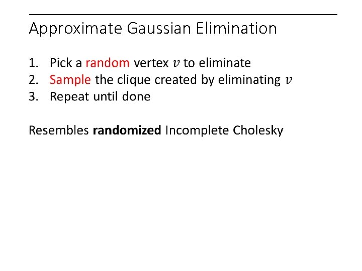
Approximate Gaussian Elimination

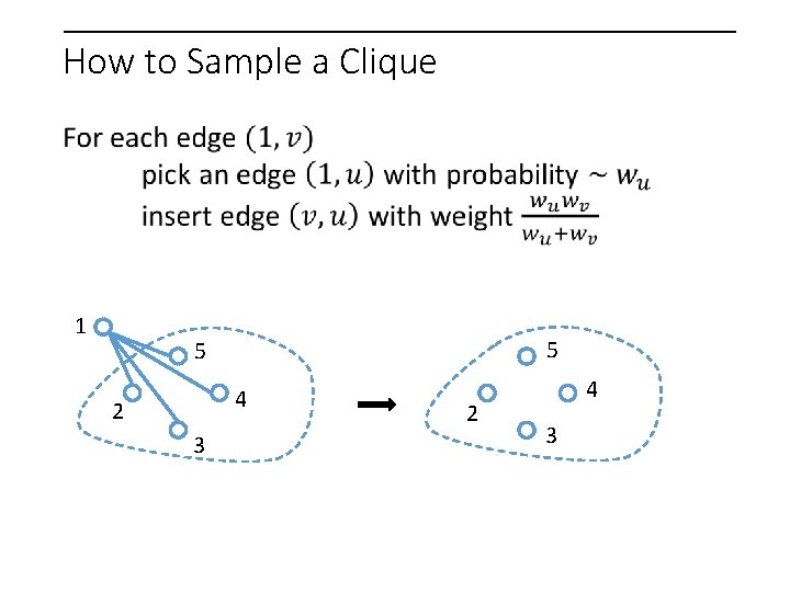
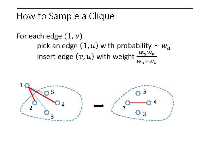
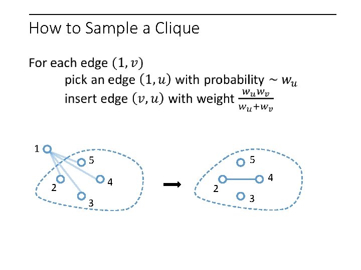
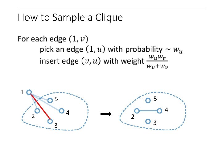
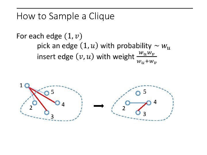
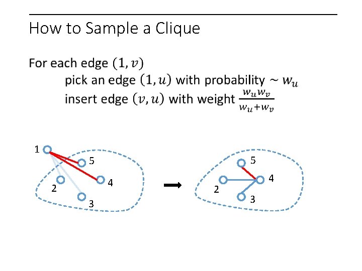
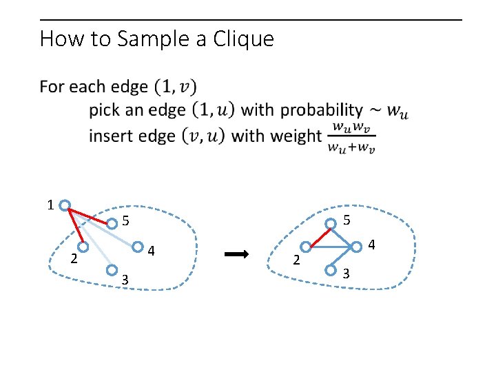
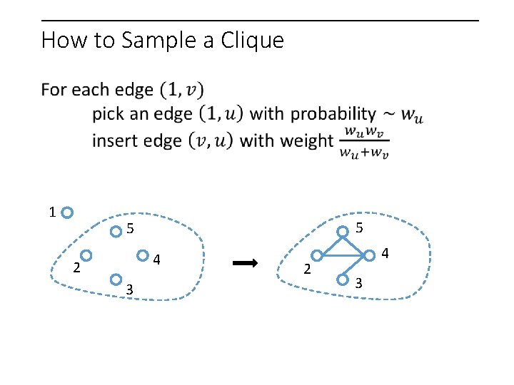
How to Sample a Clique 1 5 5 4 2 3 2 4 3

How to Sample a Clique 1 5 5 4 2 3 2 4 3

How to Sample a Clique 1 5 5 4 2 3 2 4 3

How to Sample a Clique 1 5 5 4 2 3 2 4 3

How to Sample a Clique 1 5 5 4 2 3 2 4 3

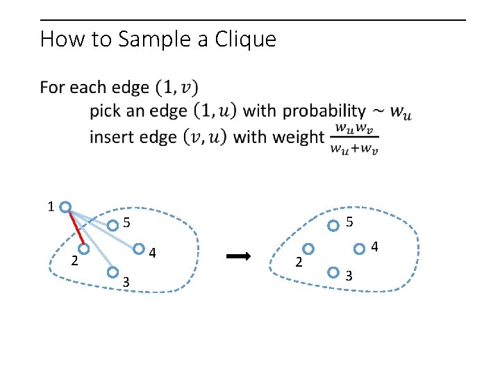
How to Sample a Clique 1 5 5 4 2 3 2 4 3

How to Sample a Clique 1 5 5 4 2 3 2 4 3

How to Sample a Clique 1 5 5 4 2 3 2 4 3

How to Sample a Clique 1 5 5 4 2 3 2 4 3

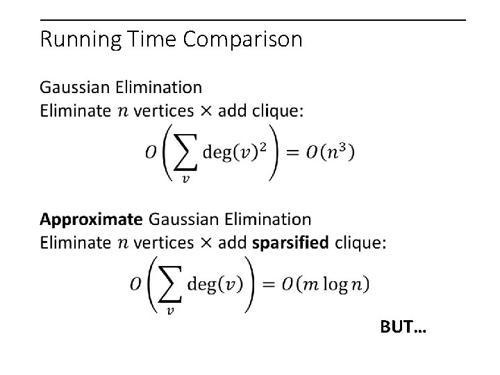
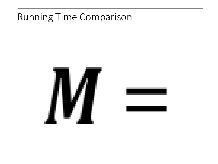
Running Time Comparison BUT…

Running Time Comparison

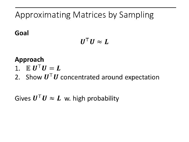
Approximating Matrices by Sampling

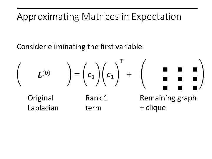
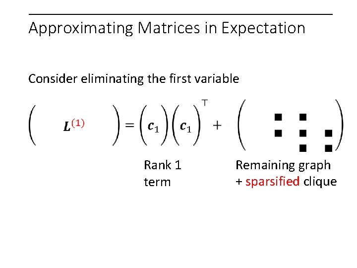
Approximating Matrices in Expectation Consider eliminating the first variable Original Laplacian Rank 1 term Remaining graph + clique

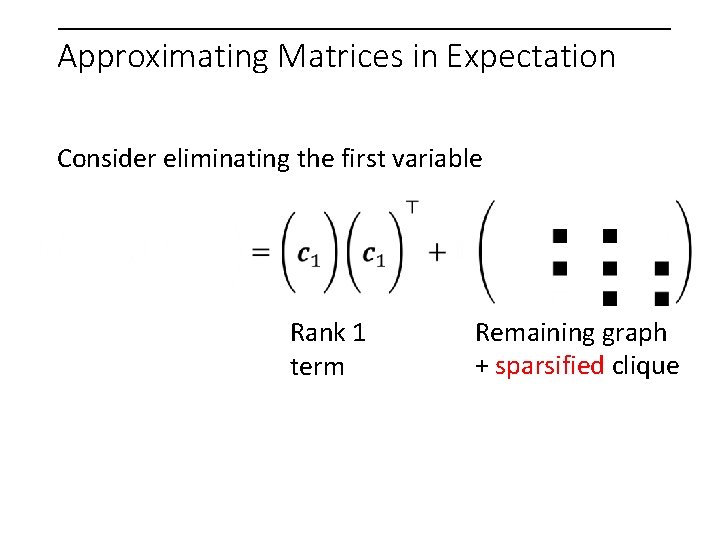
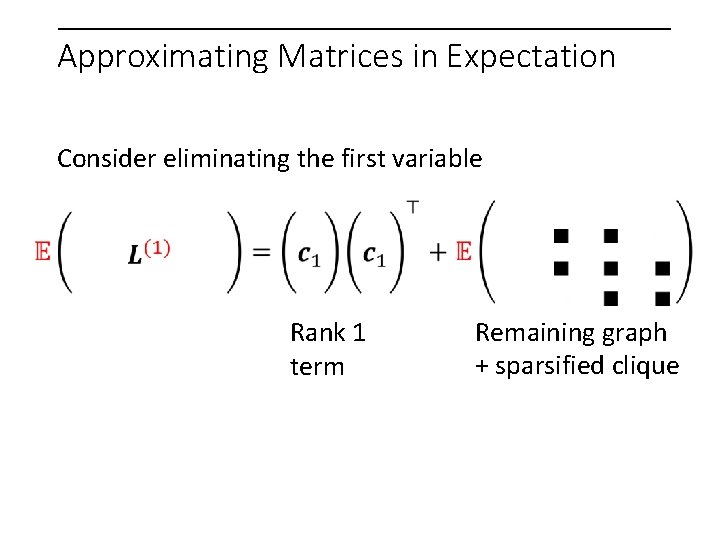
Approximating Matrices in Expectation Consider eliminating the first variable Rank 1 term Remaining graph + sparsified clique

Approximating Matrices in Expectation Consider eliminating the first variable Rank 1 term Remaining graph + sparsified clique

Approximating Matrices in Expectation Consider eliminating the first variable Rank 1 term Remaining graph + sparsified clique

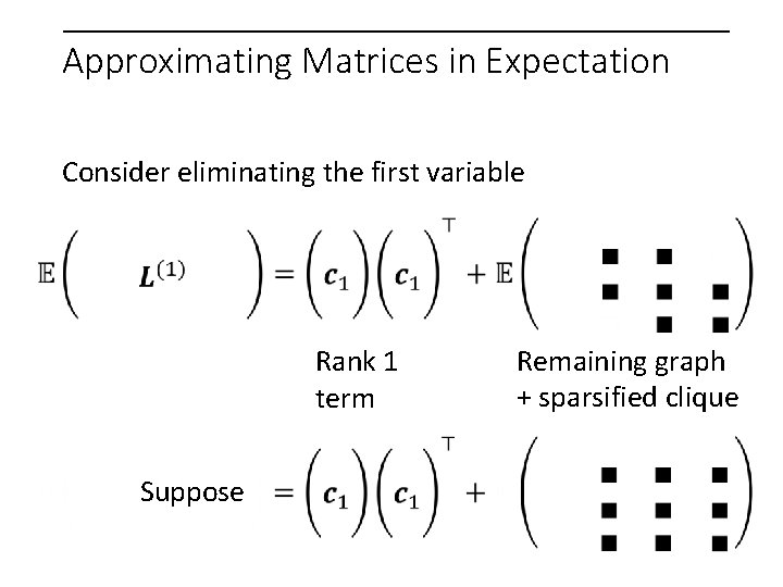
Approximating Matrices in Expectation Consider eliminating the first variable Rank 1 term Suppose Remaining graph + sparsified clique

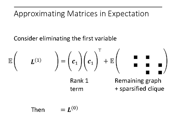
Approximating Matrices in Expectation Consider eliminating the first variable Rank 1 term Then Remaining graph + sparsified clique

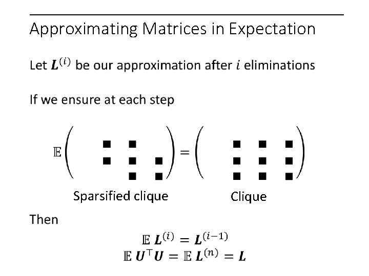
Approximating Matrices in Expectation Sparsified clique Clique

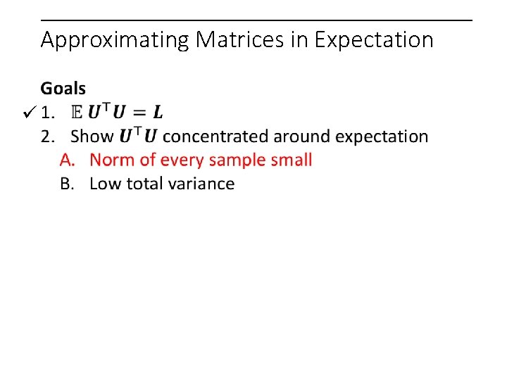
Approximating Matrices in Expectation

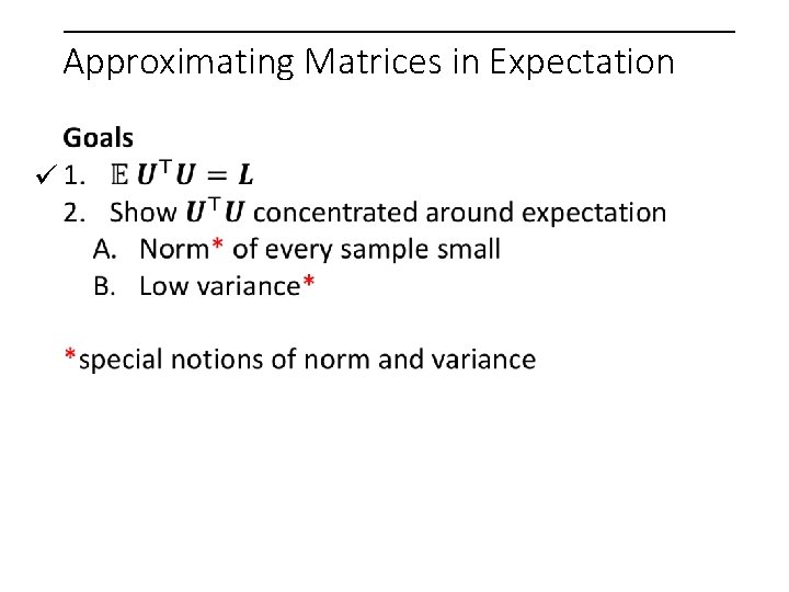
Approximating Matrices in Expectation ü

Approximating Matrices in Expectation ü

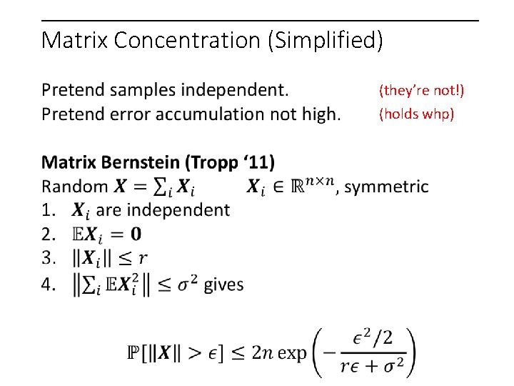
Matrix Concentration (Simplified) (they’re not!) (holds whp)

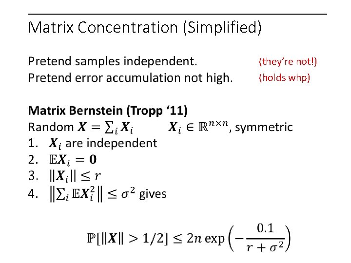
Matrix Concentration (Simplified) (they’re not!) (holds whp)

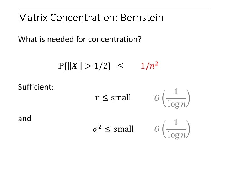
Matrix Concentration: Bernstein

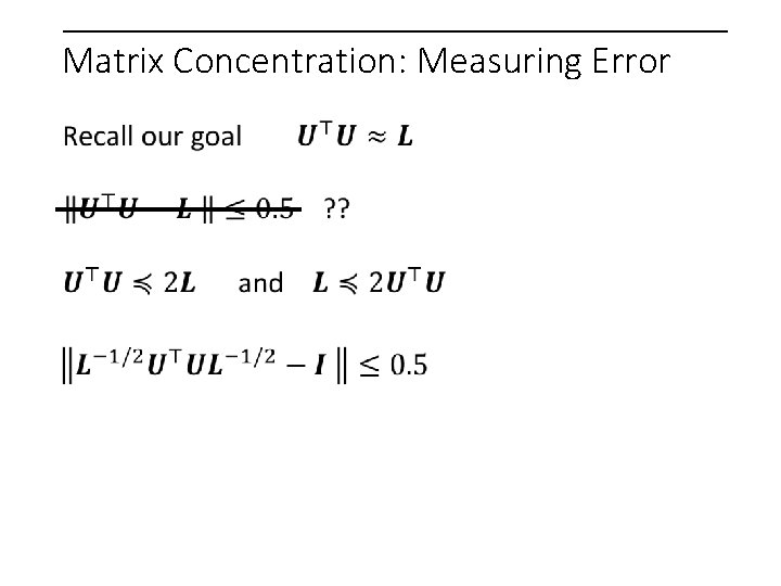
Matrix Concentration: Measuring Error

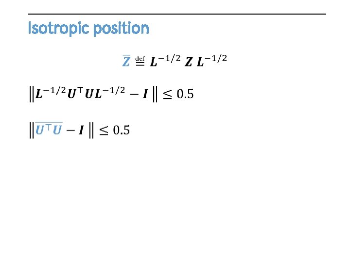
Isotropic position

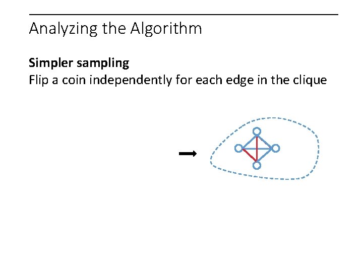
Analyzing the Algorithm Simpler sampling Flip a coin independently for each edge in the clique

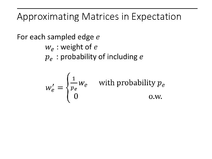
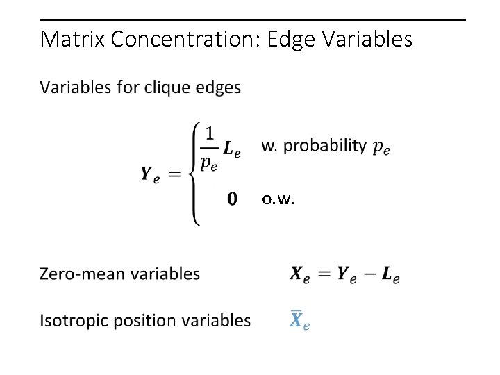
Matrix Concentration: Edge Variables o. w.

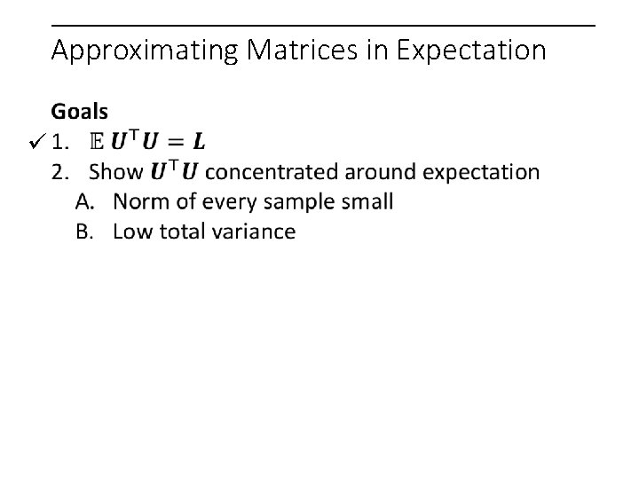
Approximating Matrices in Expectation ü

Approximating Matrices in Expectation ü

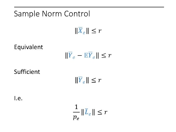
Sample Norm Control

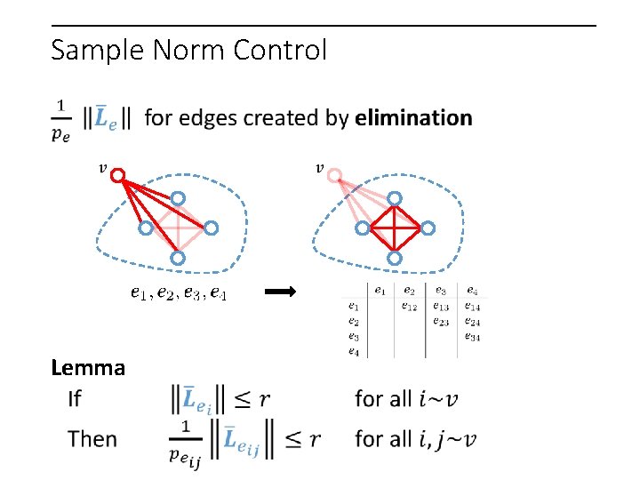
Sample Norm Control Lemma

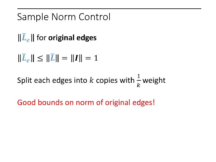
Sample Norm Control

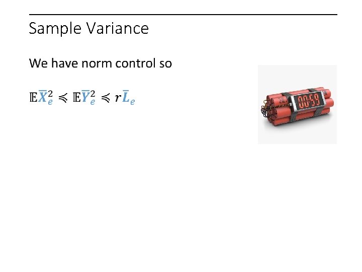
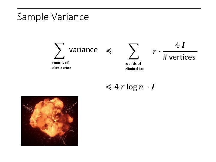
Sample Variance

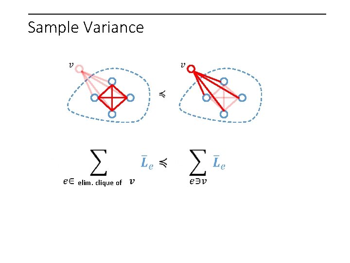
Sample Variance elim. clique of

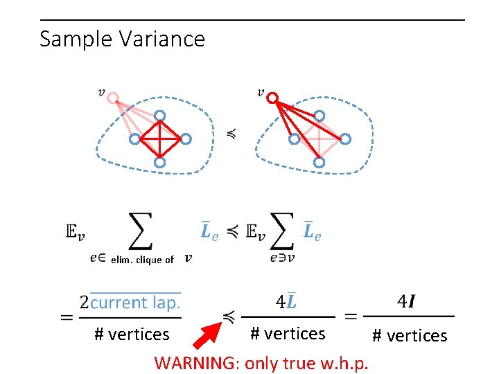
Sample Variance elim. clique of # vertices WARNING: only true w. h. p.

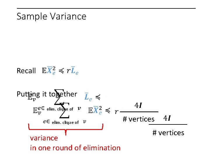
Sample Variance elim. clique of variance in one round of elimination # vertices

Sample Variance variance rounds of elimination

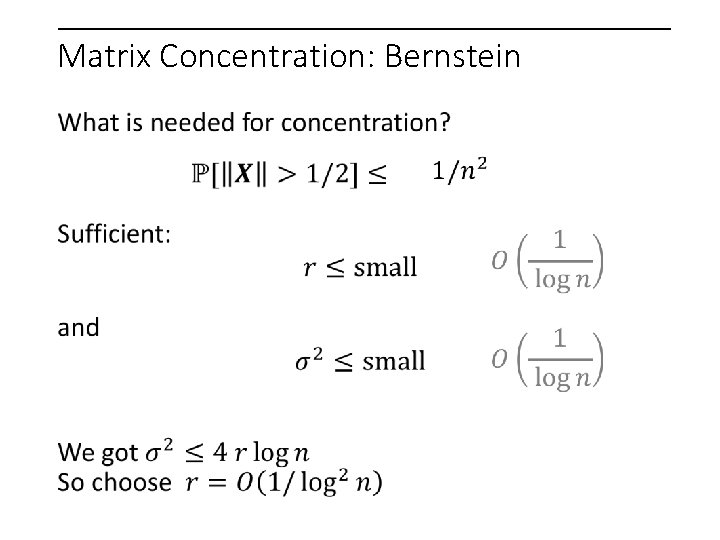
Matrix Concentration: Bernstein

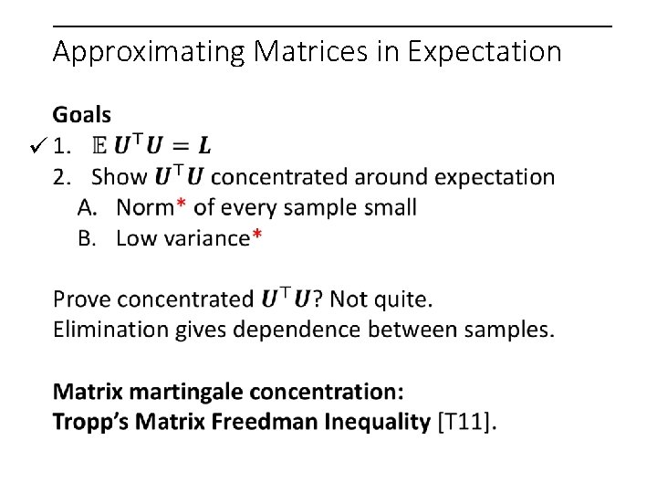
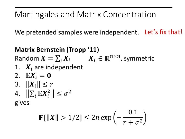
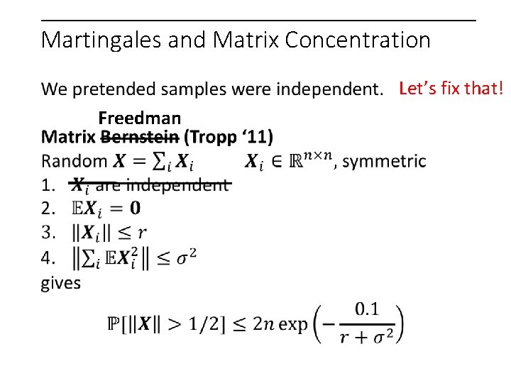
Martingales and Matrix Concentration Let’s fix that!

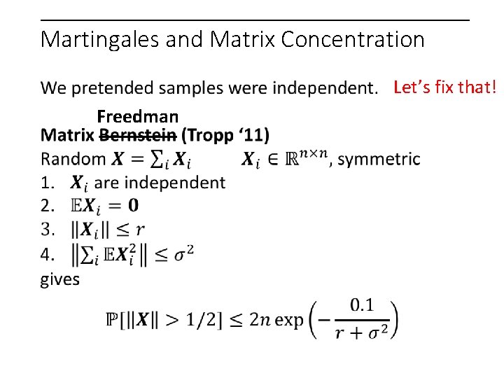
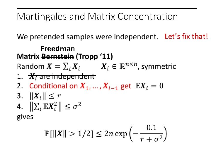
Martingales and Matrix Concentration Let’s fix that! Freedman

Martingales and Matrix Concentration Let’s fix that! Freedman

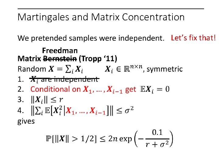
Martingales and Matrix Concentration Let’s fix that! Freedman

Martingales and Matrix Concentration Let’s fix that! Freedman

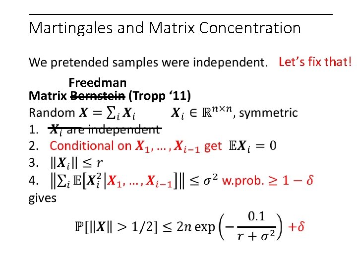
Martingales and Matrix Concentration Let’s fix that! Freedman

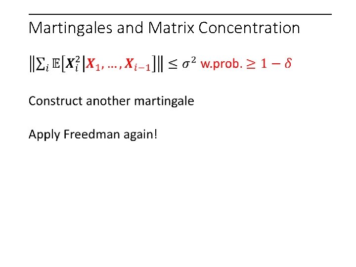
Martingales and Matrix Concentration

That’s it

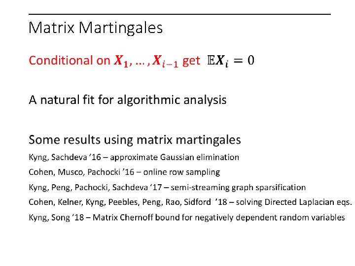
Matrix Martingales

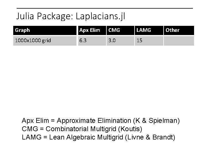
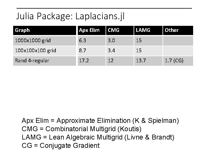
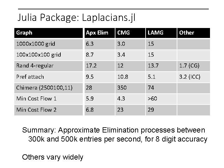
Julia Package: Laplacians. jl Graph Apx Elim CMG LAMG 1000 x 1000 grid 6. 3 3. 0 15 Other Apx Elim = Approximate Elimination (K & Spielman) CMG = Combinatorial Multigrid (Koutis) LAMG = Lean Algebraic Multigrid (Livne & Brandt)

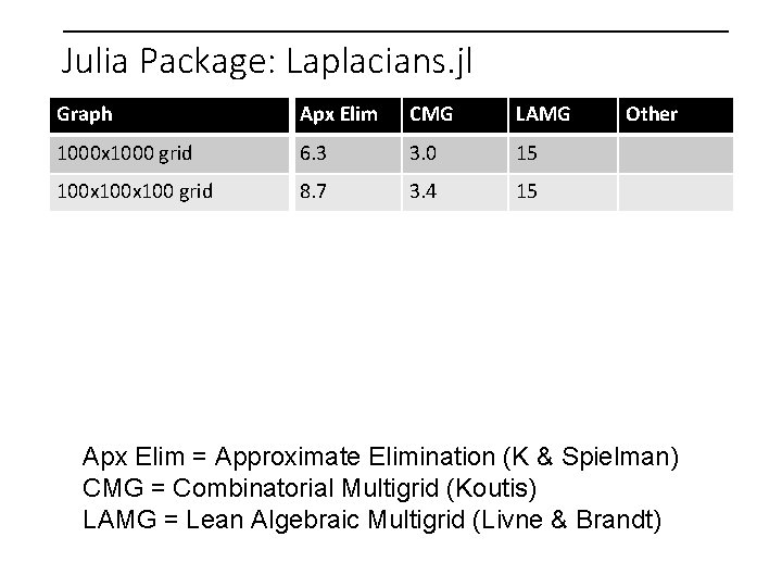
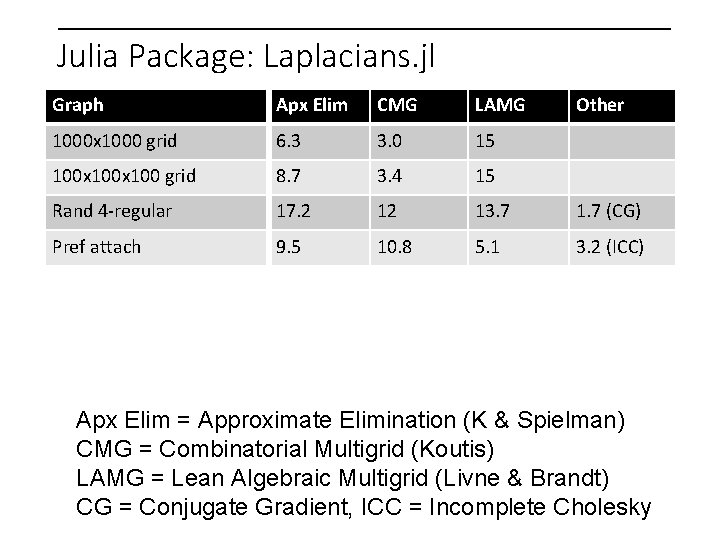
Julia Package: Laplacians. jl Graph Apx Elim CMG LAMG 1000 x 1000 grid 6. 3 3. 0 15 100 x 100 grid 8. 7 3. 4 15 Other Apx Elim = Approximate Elimination (K & Spielman) CMG = Combinatorial Multigrid (Koutis) LAMG = Lean Algebraic Multigrid (Livne & Brandt)

Julia Package: Laplacians. jl Graph Apx Elim CMG LAMG 1000 x 1000 grid 6. 3 3. 0 15 100 x 100 grid 8. 7 3. 4 15 Rand 4 -regular 17. 2 12 13. 7 Other 1. 7 (CG) Apx Elim = Approximate Elimination (K & Spielman) CMG = Combinatorial Multigrid (Koutis) LAMG = Lean Algebraic Multigrid (Livne & Brandt) CG = Conjugate Gradient

Julia Package: Laplacians. jl Graph Apx Elim CMG LAMG 1000 x 1000 grid 6. 3 3. 0 15 100 x 100 grid 8. 7 3. 4 15 Rand 4 -regular 17. 2 12 13. 7 1. 7 (CG) Pref attach 9. 5 10. 8 5. 1 3. 2 (ICC) Other Apx Elim = Approximate Elimination (K & Spielman) CMG = Combinatorial Multigrid (Koutis) LAMG = Lean Algebraic Multigrid (Livne & Brandt) CG = Conjugate Gradient, ICC = Incomplete Cholesky

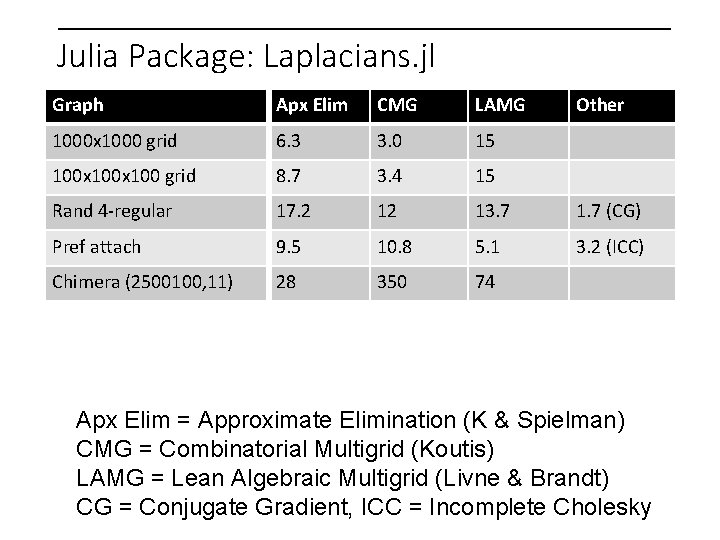
Julia Package: Laplacians. jl Graph Apx Elim CMG LAMG 1000 x 1000 grid 6. 3 3. 0 15 100 x 100 grid 8. 7 3. 4 15 Rand 4 -regular 17. 2 12 13. 7 1. 7 (CG) Pref attach 9. 5 10. 8 5. 1 3. 2 (ICC) Chimera (2500100, 11) 28 350 74 Other Apx Elim = Approximate Elimination (K & Spielman) CMG = Combinatorial Multigrid (Koutis) LAMG = Lean Algebraic Multigrid (Livne & Brandt) CG = Conjugate Gradient, ICC = Incomplete Cholesky

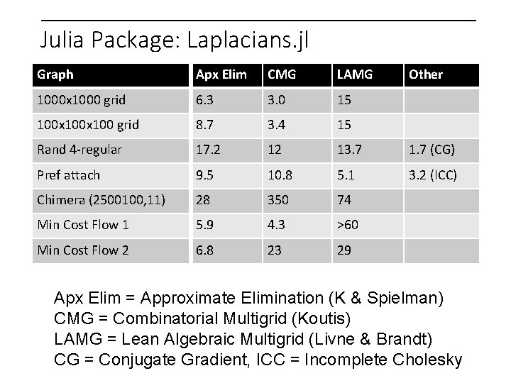
Julia Package: Laplacians. jl Graph Apx Elim CMG LAMG 1000 x 1000 grid 6. 3 3. 0 15 100 x 100 grid 8. 7 3. 4 15 Rand 4 -regular 17. 2 12 13. 7 1. 7 (CG) Pref attach 9. 5 10. 8 5. 1 3. 2 (ICC) Chimera (2500100, 11) 28 350 74 Min Cost Flow 1 5. 9 4. 3 >60 Min Cost Flow 2 6. 8 23 29 Other Apx Elim = Approximate Elimination (K & Spielman) CMG = Combinatorial Multigrid (Koutis) LAMG = Lean Algebraic Multigrid (Livne & Brandt) CG = Conjugate Gradient, ICC = Incomplete Cholesky

Julia Package: Laplacians. jl Graph Apx Elim CMG LAMG 1000 x 1000 grid 6. 3 3. 0 15 100 x 100 grid 8. 7 3. 4 15 Rand 4 -regular 17. 2 12 13. 7 1. 7 (CG) Pref attach 9. 5 10. 8 5. 1 3. 2 (ICC) Chimera (2500100, 11) 28 350 74 Min Cost Flow 1 5. 9 4. 3 >60 Min Cost Flow 2 6. 8 23 29 Other Summary: Approximate Elimination processes between 300 k and 500 k entries per second, for 8 digit accuracy Others vary widely

Thanks!

This is really the end

Older slides