Fast Exact and Approximate Geodesics on Meshes Vitaly

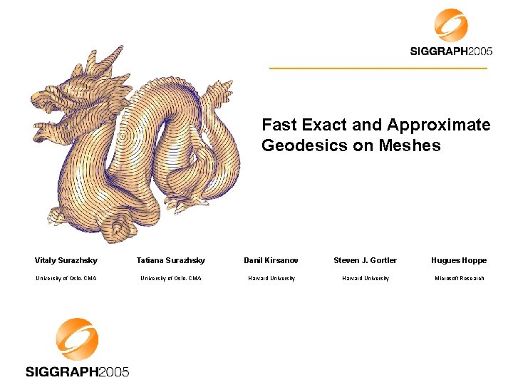
Fast Exact and Approximate Geodesics on Meshes Vitaly Surazhsky Tatiana Surazhsky Danil Kirsanov Steven J. Gortler Hugues Hoppe University of Oslo, CMA Harvard University Microsoft Research

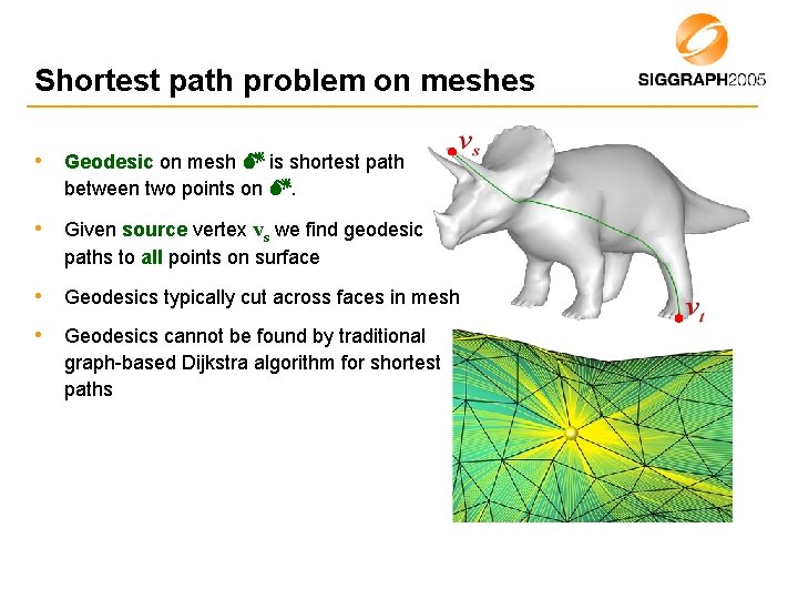
Shortest path problem on meshes • Geodesic on mesh is shortest path between two points on . • Given source vertex vs we find geodesic paths to all points on surface • Geodesics typically cut across faces in mesh • Geodesics cannot be found by traditional graph-based Dijkstra algorithm for shortest paths

Outline • Introduction • The algorithm computing exact shortest paths and distances on a triangular mesh (Mitchell et. al. [1987]) • Approximation algorithm • Exact geodesic between two vertices • Experimental results • Conclusions

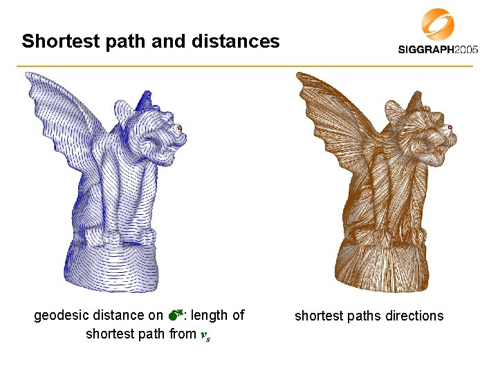
Shortest path and distances geodesic distance on : length of shortest path from vs shortest paths directions

Motivation • Shortest paths: – Mesh partitioning (for atlas parameterization) [Krishnamurthy and Levoy 1996; Sander et al. 2003] – Mesh segmentation [Katz and Tal 2003; Funkhouser et al. 2004] – Mesh editing (delineating edit operation) [Kobbelt et al. 1998] • Shortest distance metric – radial-basis interpolation over mesh – skinning [Sloan et al. 2001]; – mesh watermarking [Praun et al. 1999]

Previous work – exact geodesics • Mitchell, Mount, Papadimitriou [MMP 1987] – worst case complexity: O(n 2 log n) – never implemented • Chen and Han [1996] – complexity O(n 2) – partially implemented by Kaneva and O’Rourke [2000] • Kapoor [1999] – “single source, single destination” – complexity: O(n log 2 n)

Previous work – approximate geodesics • Lanthier et al. [1997] – guaranteed error bounds – by adding extra edges • Kanai and Suzuki [2001]; Martinez et al. [2004] – iterative optimization (depends on initial approximate path) • Kimmel and Sethian [1998]: fast marching method – require special processing of triangles with obtuse angles – time complexity: O(n log n) • Novotni and Klein [2002]; Kirsanov [2004]; Reimers [2004] – employ improved update rule • Polthier and Schmies [1998] – “straightest path” …

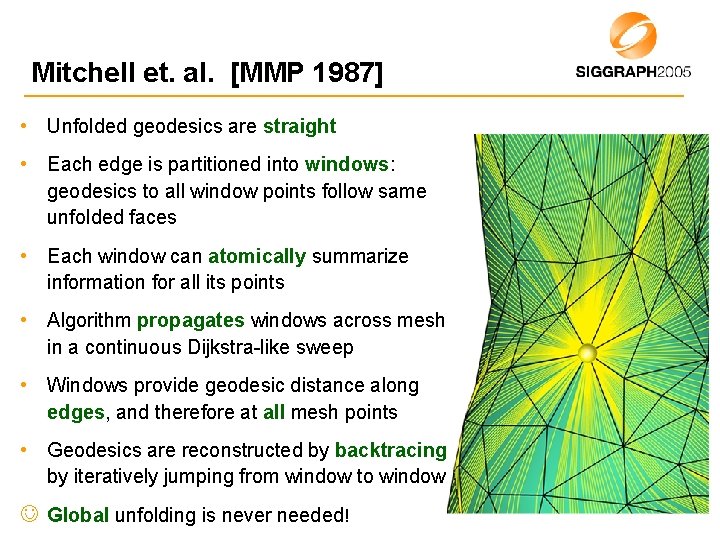
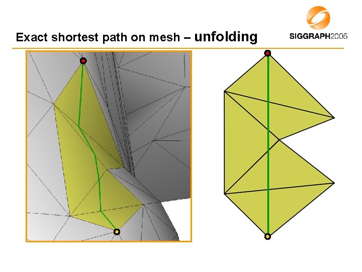
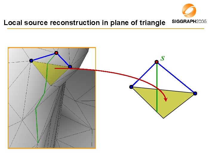
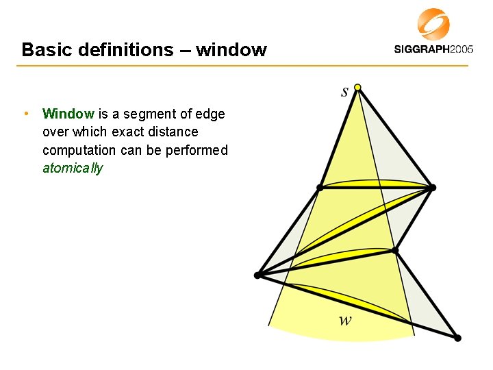
Mitchell et. al. [MMP 1987] • Unfolded geodesics are straight • Each edge is partitioned into windows: geodesics to all window points follow same unfolded faces • Each window can atomically summarize information for all its points • Algorithm propagates windows across mesh in a continuous Dijkstra-like sweep • Windows provide geodesic distance along edges, and therefore at all mesh points • Geodesics are reconstructed by backtracing by iteratively jumping from window to window J Global unfolding is never needed!

Exact shortest path on mesh – unfolding

Local source reconstruction in plane of triangle

Basic definitions – window • Window is a segment of edge over which exact distance computation can be performed atomically

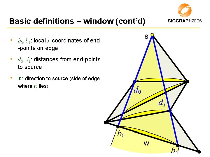
Basic definitions – window (cont’d) • b 0, b 1: local x-coordinates of end -points on edge • d 0, d 1: distances from end-points to source • : direction to source (side of edge where vs lies)

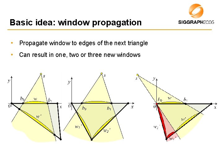
Basic idea: window propagation • Propagate window to edges of the next triangle • Can result in one, two or three new windows

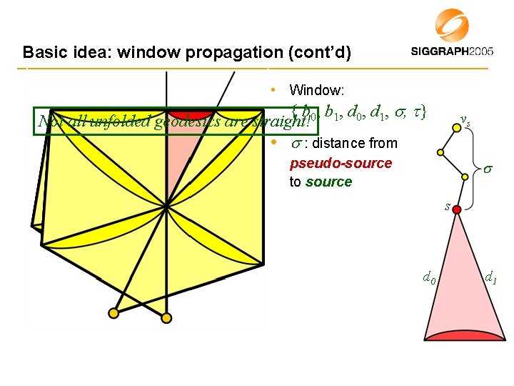
Basic idea: window propagation (cont’d) • Window: { b 0, b 1, d 0, d 1, , } Not all unfolded geodesics are straight! vs • : distance from pseudo-source to source s d 0 d 1

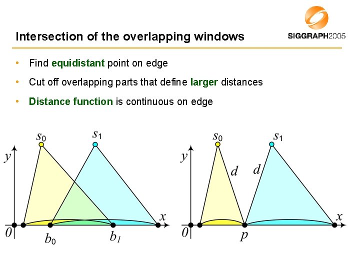
Intersection of the overlapping windows • Find equidistant point on edge • Cut off overlapping parts that define larger distances • Distance function is continuous on edge

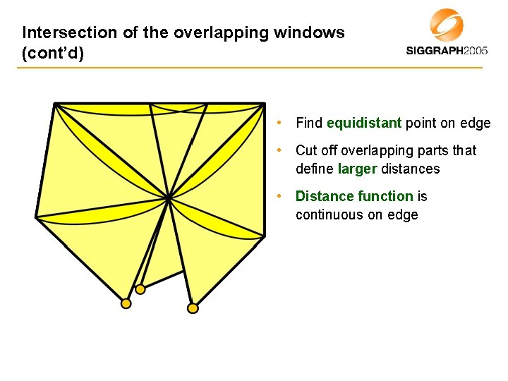
Intersection of the overlapping windows (cont’d) • Find equidistant point on edge • Cut off overlapping parts that define larger distances • Distance function is continuous on edge

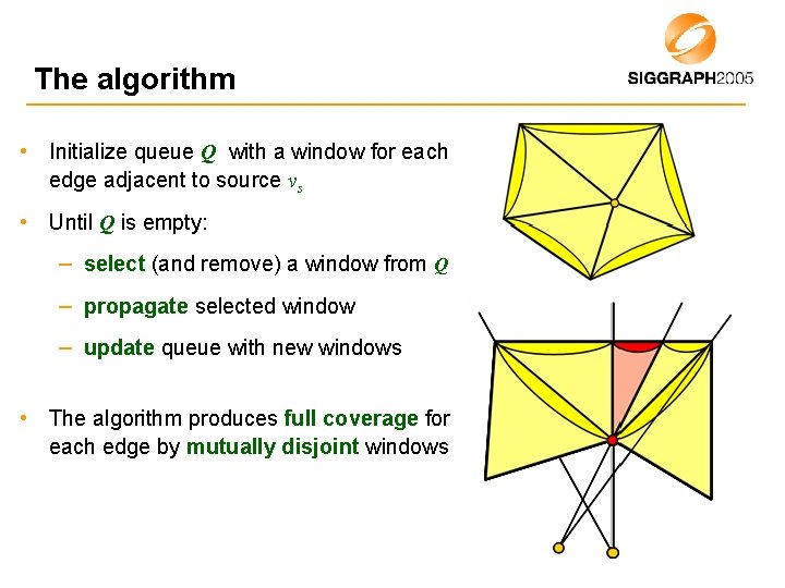
The algorithm • Initialize queue Q with a window for each edge adjacent to source vs • Until Q is empty: – select (and remove) a window from Q – propagate selected window – update queue with new windows • The algorithm produces full coverage for each edge by mutually disjoint windows

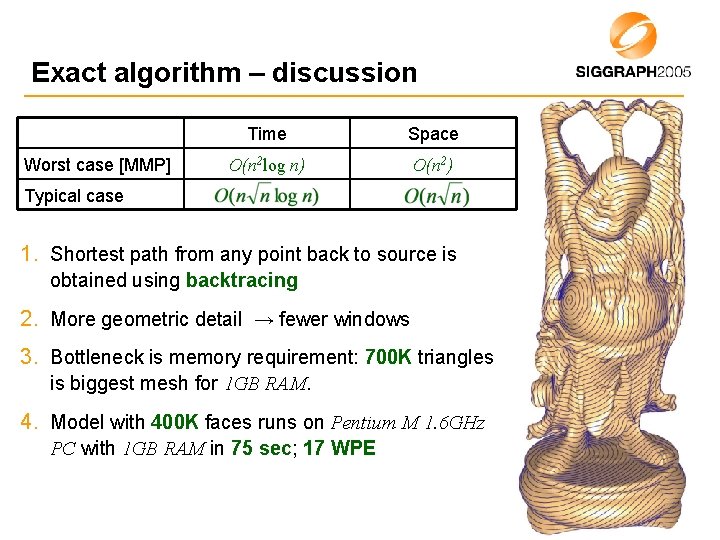
Exact algorithm – discussion Worst case [MMP] Time Space O(n 2 log n) O(n 2) Typical case 1. Shortest path from any point back to source is obtained using backtracing 2. More geometric detail → fewer windows 3. Bottleneck is memory requirement: 700 K triangles is biggest mesh for 1 GB RAM. 4. Model with 400 K faces runs on Pentium M 1. 6 GHz PC with 1 GB RAM in 75 sec; 17 WPE

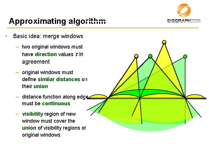
Approximating algorithm • Basic idea: merge windows – two original windows must have direction values in agreement – original windows must define similar distances on their union – distance function along edge must be continuous – visibility region of new window must cover the union of visibility regions of original windows

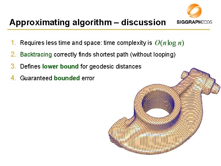
Approximating algorithm – discussion 1. Requires less time and space: time complexity is 2. Backtracing correctly finds shortest path (without looping) 3. Defines lower bound for geodesic distances 4. Guaranteed bounded error

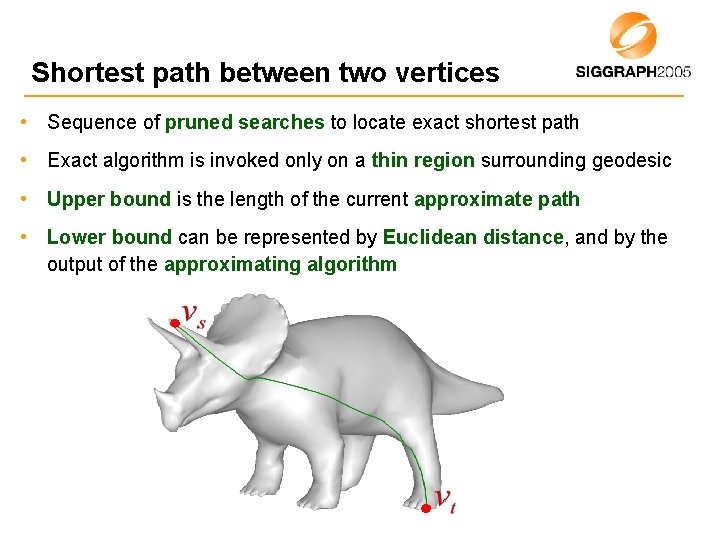
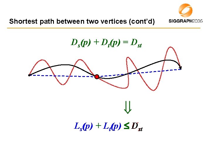
Shortest path between two vertices • Sequence of pruned searches to locate exact shortest path • Exact algorithm is invoked only on a thin region surrounding geodesic • Upper bound is the length of the current approximate path • Lower bound can be represented by Euclidean distance, and by the output of the approximating algorithm

Shortest path between two vertices (cont’d) Ds(p) + Dt(p) = Dst Ls(p) + Lt(p) U Dst

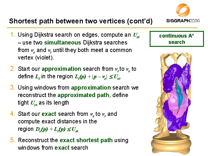
Shortest path between two vertices (cont’d) 1. Using Dijkstra search on edges, compute an Ust – use two simultaneous Dijkstra searches from vs and vt until they both meet a common vertex (violet). 2. Start our approximation search from vt to vs to define Lt in the region Lt(p) + |p – vs| Ust 3. Using windows from approximation search we reconstruct the approximated path, define tight Ust as its length 4. Start our exact search from vs to vt and compute exact distances in the region Ds(p) + Lt(p) Ust 5. Reconstruct the exact shortest path using windows from exact search continuous A* search

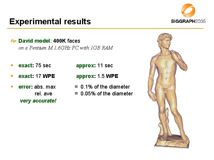
Experimental results David model: 400 K faces on a Pentium M 1. 6 GHz PC with 1 GB RAM § exact: 75 sec approx: 11 sec § exact: 17 WPE approx: 1. 5 WPE § error: abs. max = 0. 1% of the diameter = 0. 05% of the diameter rel. ave very accurate!

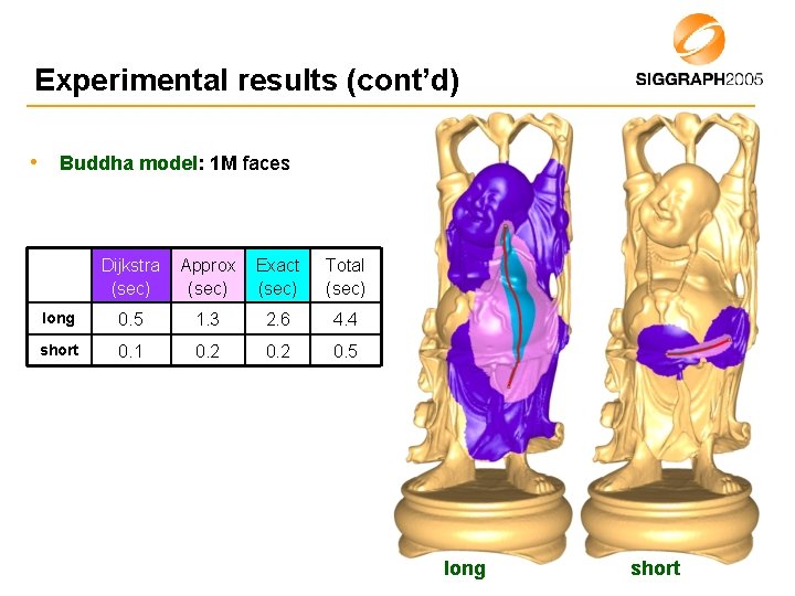
Experimental results (cont’d) • Buddha model: 1 M faces Dijkstra (sec) Approx (sec) Exact (sec) Total (sec) long 0. 5 1. 3 2. 6 4. 4 short 0. 1 0. 2 0. 5 long short

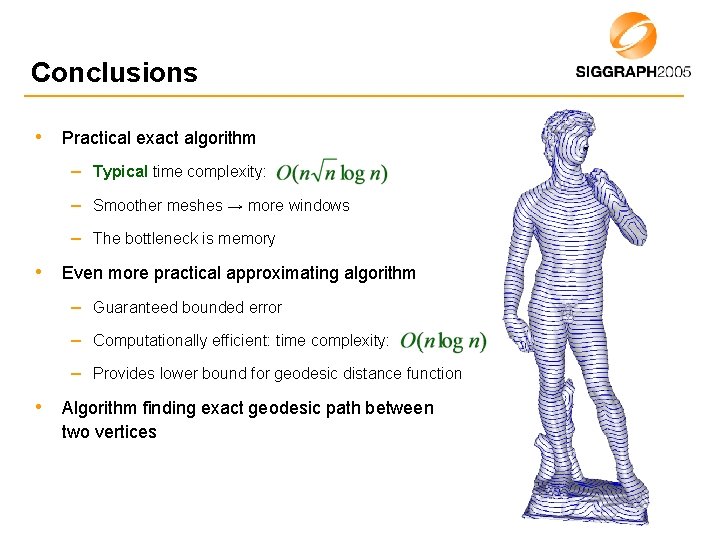
Conclusions • Practical exact algorithm – Typical time complexity: – Smoother meshes → more windows – The bottleneck is memory • Even more practical approximating algorithm – Guaranteed bounded error – Computationally efficient: time complexity: – Provides lower bound for geodesic distance function • Algorithm finding exact geodesic path between two vertices

Thank you!