Parallel Gaussian Elimination 2 D Mapping with Pipelining

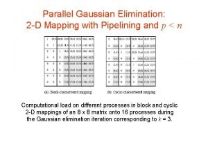
Parallel Gaussian Elimination: 2 -D Mapping with Pipelining and p < n Computational load on different processes in block and cyclic 2 -D mappings of an 8 x 8 matrix onto 16 processes during the Gaussian elimination iteration corresponding to k = 3.

Parallel Gaussian Elimination: 2 -D Cyclic Mapping • The idling in the block mapping can be alleviated using a cyclic mapping. • The maximum difference in computational load between any two processes in any iteration is that of one row and one column update. • This contributes to the overhead function. Since there are n iterations, the total overhead is .

Gaussian Elimination with Partial Pivoting • For numerical stability, one generally uses partial pivoting. • In the k th iteration, we select a column i (called the pivot column) such that A[k, i] is the largest in magnitude among all A[k, i] such that k ≤ j < n. • The k th and the i th columns are interchanged. • Simple to implement with row-partitioning and does not add overhead since the division step takes the same time as computing the max. • Column-partitioning, however, requires a global reduction, adding a log p term to the overhead. • Pivoting precludes the use of pipelining.

Gaussian Elimination with Partial Pivoting: 2 D Partitioning • Partial pivoting restricts use of pipelining, resulting in performance loss. • This loss can be alleviated by restricting pivoting to specific columns. • Alternately, we can use faster algorithms for broadcast.

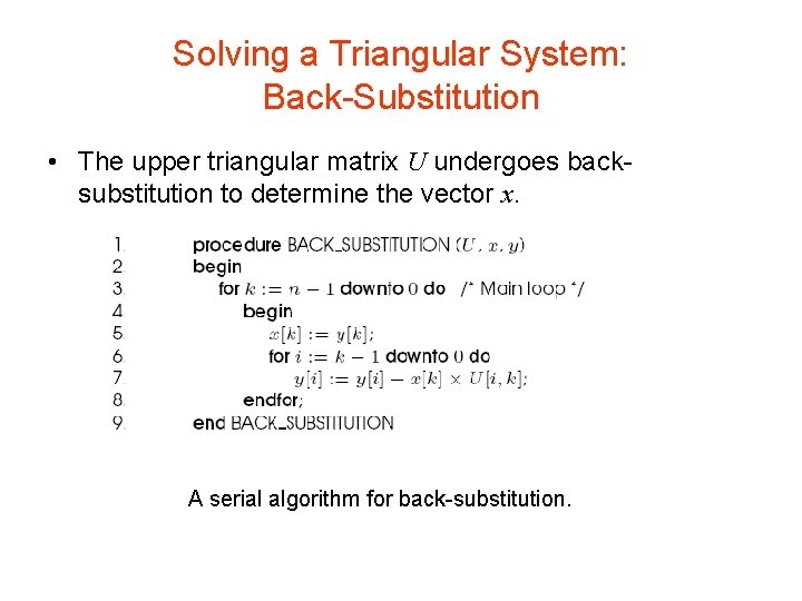
Solving a Triangular System: Back-Substitution • The upper triangular matrix U undergoes backsubstitution to determine the vector x. A serial algorithm for back-substitution.

Solving a Triangular System: Back-Substitution • The algorithm performs approximately n 2/2 multiplications and subtractions. • Since complexity of this part is asymptotically lower, we should optimize the data distribution for the factorization part. • Consider a rowwise block 1 -D mapping of the n x n matrix U with vector y distributed uniformly. • The value of the variable solved at a step can be pipelined back. • Each step of a pipelined implementation requires a constant amount of time for communication and Θ(n/p) time for computation. • The parallel run time of the entire algorithm is Θ(n 2/p).

Solving a Triangular System: Back-Substitution • If the matrix is partitioned by using 2 -D partitioning on a logical mesh of processes, and the elements of the vector are distributed along one of the columns of the process mesh, then only the processes containing the vector perform any computation. • Using pipelining to communicate the appropriate elements of U to the process containing the corresponding elements of y for the substitution step (line 7), the algorithm can be executed in time. • While this is not cost optimal, since this does not dominate the overall computation, the cost optimality is determined by the factorization.