NECSI Summer School 2008 Week 3 Methods for

NECSI Summer School 2008 Week 3: Methods for the Study of Complex Systems Analytical Tools for Dynamical Systems Hiroki Sayama sayama@binghamton. edu

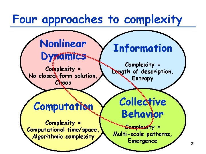
Four approaches to complexity Nonlinear Dynamics Complexity = No closed-form solution, Chaos Computation Complexity = Computational time/space, Algorithmic complexity Information Complexity = Length of description, Entropy Collective Behavior Complexity = Multi-scale patterns, Emergence 2

Local Linearization and Linear Stability Analysis 3

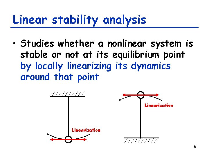
Stability of equilibrium points • If a system at its equilibrium point is slightly perturbed, what happens? • The equilibrium point is called: – Stable (or asymptotically stable) if the system eventually falls back to the equilibrium point – Lyapunov stable if the system doesn’t go far away from the equilibrium point – Unstable otherwise 4

Question • What is the stability of each of the following equilibrium points? 5

Linear stability analysis • Studies whether a nonlinear system is stable or not at its equilibrium point by locally linearizing its dynamics around that point Linearization 6

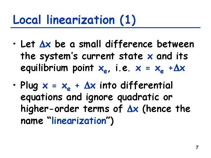
Local linearization (1) • Let Dx be a small difference between the system’s current state x and its equilibrium point xe, i. e. x = xe +Dx • Plug x = xe + Dx into differential equations and ignore quadratic or higher-order terms of Dx (hence the name “linearization”) 7

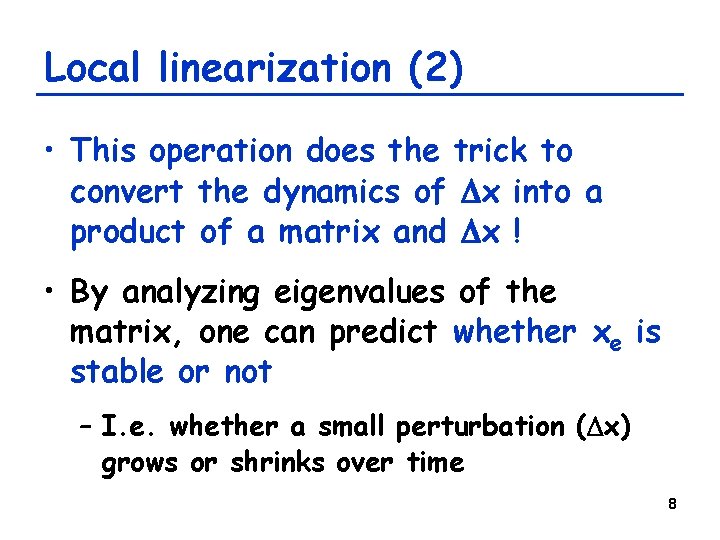
Local linearization (2) • This operation does the trick to convert the dynamics of Dx into a product of a matrix and Dx ! • By analyzing eigenvalues of the matrix, one can predict whether xe is stable or not – I. e. whether a small perturbation (Dx) grows or shrinks over time 8

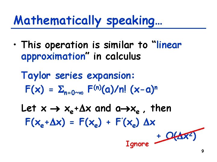
Mathematically speaking… • This operation is similar to “linear approximation” in calculus Taylor series expansion: F(x) = Sn=0~ F(n)(a)/n! (x-a)n Let x xe+Dx and a xe , then F(xe+Dx) = F(xe) + F’(xe) Dx + O(Dx 2) Ignore 9

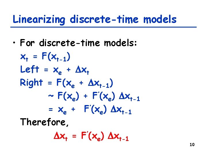
Linearizing discrete-time models • For discrete-time models: xt = F(xt-1) Left = xe + Dxt Right = F(xe + Dxt-1) ~ F(xe) + F’(xe) Dxt-1 = xe + F’(xe) Dxt-1 Therefore, Dxt = F’(xe) Dxt-1 10

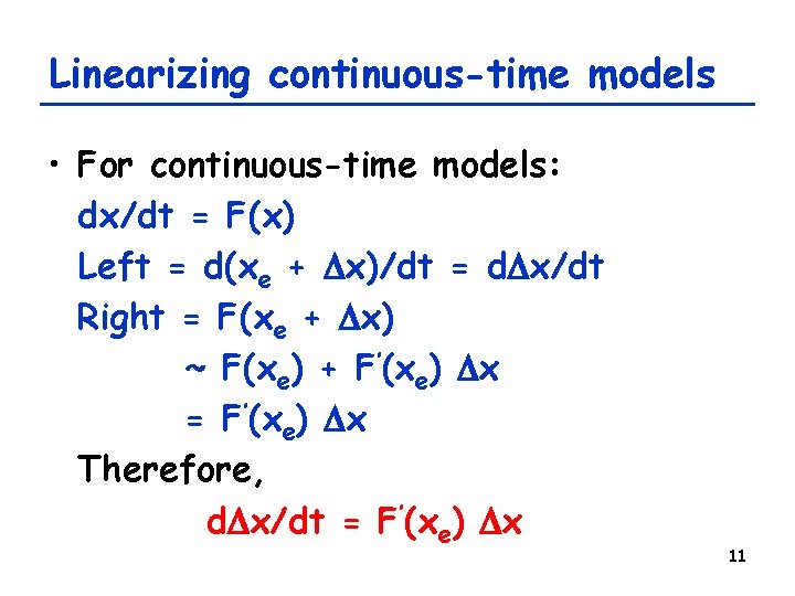
Linearizing continuous-time models • For continuous-time models: dx/dt = F(x) Left = d(xe + Dx)/dt = d. Dx/dt Right = F(xe + Dx) ~ F(xe) + F’(xe) Dx = F’(xe) Dx Therefore, d. Dx/dt = F’(xe) Dx 11

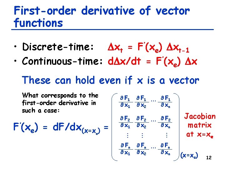
First-order derivative of vector functions • Discrete-time: Dxt = F’(xe) Dxt-1 • Continuous-time: d. Dx/dt = F’(xe) Dx These can hold even if x is a vector What corresponds to the first-order derivative in such a case: F 2 x 1 F 2 … x 2 xn … Fn x 1 … e F 1 … x 2 xn … F’(xe) = d. F/dx(x=x ) = F 1 x 1 Fn … Fn x 2 xn Jacobian matrix at x=xe (x=xe) 12

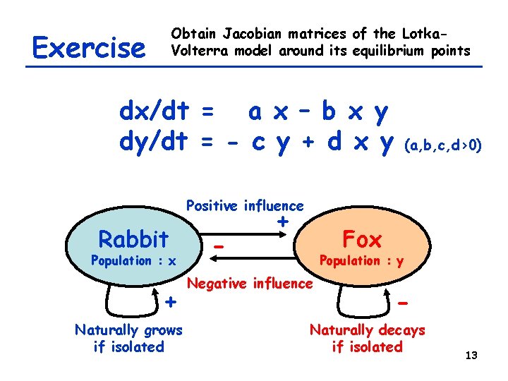
Obtain Jacobian matrices of the Lotka. Volterra model around its equilibrium points Exercise dx/dt = a x – b x y dy/dt = - c y + d x y (a, b, c, d>0) Positive influence Rabbit Population : x + Naturally grows if isolated - + Fox Population : y Negative influence - Naturally decays if isolated 13

Eigenvalues of Jacobian matrix • A Jacobian matrix is a linear approximation around the equilibrium point, telling you the local dynamics: “how a small perturbation will grow, shrink or rotate around that point” – The equilibrium point serves as a local origin – The Dx serves as a local coordinate – Eigenvalue analysis applies 14

Review: What eigenvalues and eigenvectors can tell us • An eigenvalue tells whether a particular “state” of the system (specified by its corresponding eigenvectors) grows or shrinks by interactions between parts – | l | > 1 -> growing for discrete-time cases – | l | < 1 -> shrinking – Re(l) > 0 -> growing for continuous-time cases – Re(l) < 0 -> shrinking 15

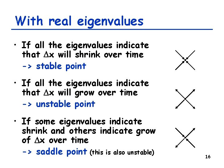
With real eigenvalues • If all the eigenvalues indicate that Dx will shrink over time -> stable point • If all the eigenvalues indicate that Dx will grow over time -> unstable point • If some eigenvalues indicate shrink and others indicate grow of Dx over time -> saddle point (this is also unstable) 16

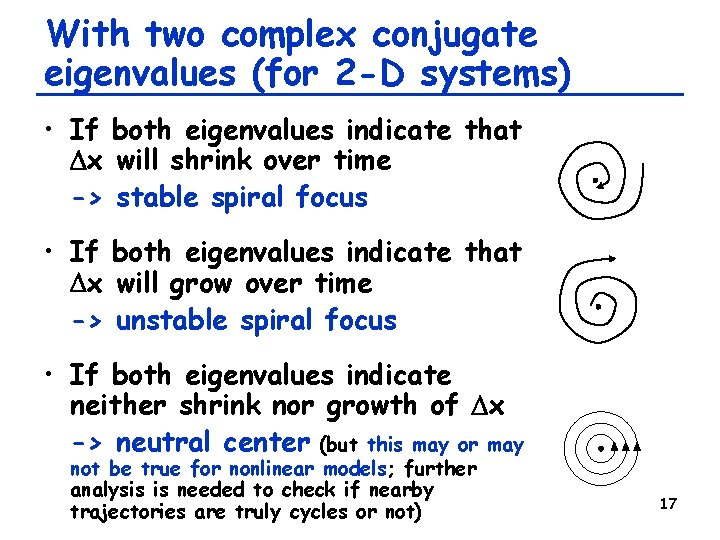
With two complex conjugate eigenvalues (for 2 -D systems) • If both eigenvalues indicate that Dx will shrink over time -> stable spiral focus • If both eigenvalues indicate that Dx will grow over time -> unstable spiral focus • If both eigenvalues indicate neither shrink nor growth of Dx -> neutral center (but this may or may not be true for nonlinear models; further analysis is needed to check if nearby trajectories are truly cycles or not) 17

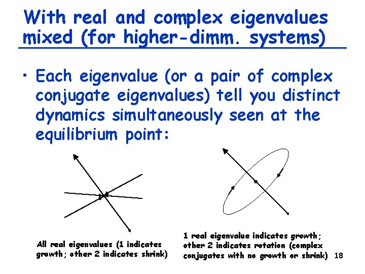
With real and complex eigenvalues mixed (for higher-dimm. systems) • Each eigenvalue (or a pair of complex conjugate eigenvalues) tell you distinct dynamics simultaneously seen at the equilibrium point: All real eigenvalues (1 indicates growth; other 2 indicates shrink) 1 real eigenvalue indicates growth; other 2 indicates rotation (complex conjugates with no growth or shrink) 18

Exercise • Evaluate the stabilities of equilibrium points of the Lotka-Volterra model using eigenvalue analysis of Jacobian matrices • Do the same analysis for the revised version with carrying capacity and upper bound of predation rate 19

Bifurcations 20

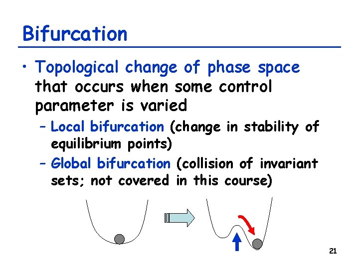
Bifurcation • Topological change of phase space that occurs when some control parameter is varied – Local bifurcation (change in stability of equilibrium points) – Global bifurcation (collision of invariant sets; not covered in this course) 21

Bifurcations in complex systems • Often play important roles as a switching mechanism that causes abrupt changes of systems’ behavior from one to another – Conformation switching of proteins and other biopolymers – Neural switching (resting/excited) – Pattern formation in morphogenesis (will be discussed later) 22

When bifurcation occurs in nonlinear systems • { li }: eigenvalues of Jacobian matrix at equilibrium point xe • xe is: – Stable if |li| < 1 for all i or if Re(li) < 0 for all i – Unstable if |li| > 1 for some i or if Re(li) > 0 for some i (discrete-time) (continuous-time) • Bifurcation occurs when the above inequalities become equations, i. e. , when the stability of an equilibrium point changes – |li| = 1 or Re(li) = 0, for some i (discrete-time) (continuous-time) 23

Bifurcations in 1 -D Systems 24

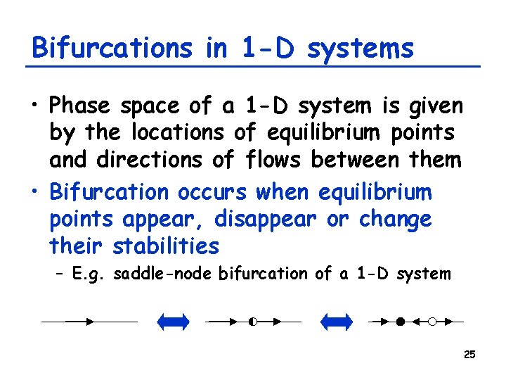
Bifurcations in 1 -D systems • Phase space of a 1 -D system is given by the locations of equilibrium points and directions of flows between them • Bifurcation occurs when equilibrium points appear, disappear or change their stabilities – E. g. saddle-node bifurcation of a 1 -D system 25

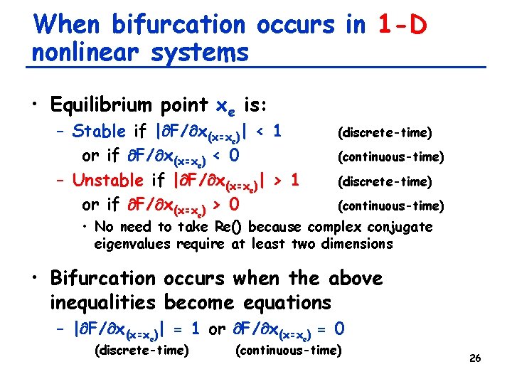
When bifurcation occurs in 1 -D nonlinear systems • Equilibrium point xe is: – Stable if | F/ x(x=xe)| < 1 or if F/ x(x=xe) < 0 – Unstable if | F/ x(x=xe)| > 1 or if F/ x(x=xe) > 0 (discrete-time) (continuous-time) • No need to take Re() because complex conjugate eigenvalues require at least two dimensions • Bifurcation occurs when the above inequalities become equations – | F/ x(x=xe)| = 1 or F/ x(x=xe) = 0 (discrete-time) (continuous-time) 26

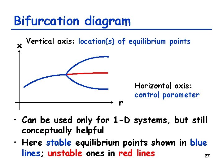
Bifurcation diagram x Vertical axis: location(s) of equilibrium points r Horizontal axis: control parameter • Can be used only for 1 -D systems, but still conceptually helpful • Here stable equilibrium points shown in blue lines; unstable ones in red lines 27

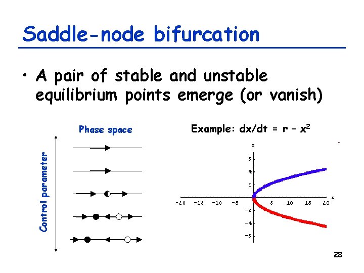
Saddle-node bifurcation • A pair of stable and unstable equilibrium points emerge (or vanish) Example: dx/dt = r – x 2 Control parameter Phase space 28

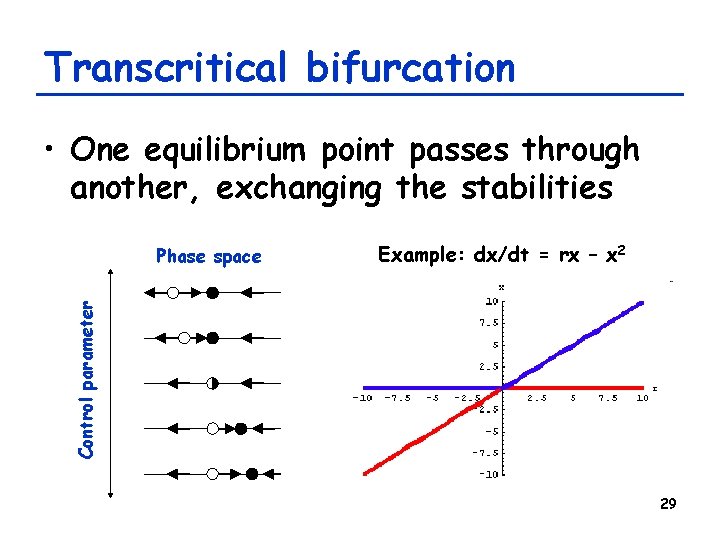
Transcritical bifurcation • One equilibrium point passes through another, exchanging the stabilities Example: dx/dt = rx – x 2 Control parameter Phase space 29

Pitchfork bifurcation • A stable point splits into two (with one unstable point also emerging) Example: dx/dt = rx – x 3 Control parameter Phase space 30

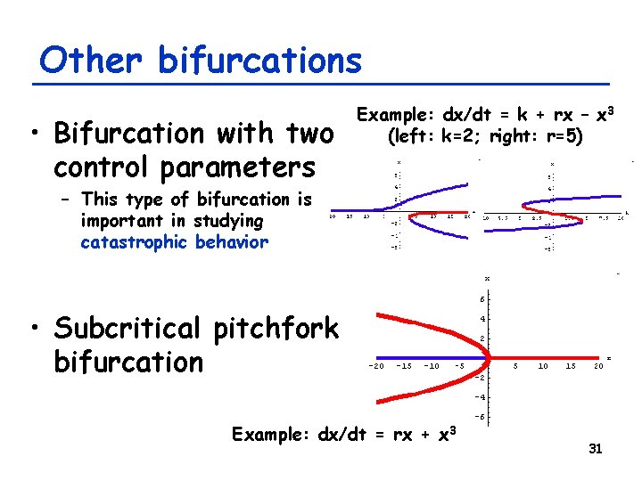
Other bifurcations • Bifurcation with two control parameters Example: dx/dt = k + rx – x 3 (left: k=2; right: r=5) – This type of bifurcation is important in studying catastrophic behavior • Subcritical pitchfork bifurcation Example: dx/dt = rx + x 3 31

Exercise: Two competing species • Two species “x” and “y” compete for a finite resource or habitat • Total population is assumed constant x + y = K (i. e. , the systems is 1 -D) • Growth is influenced by their relative population difference: dx/dt = a x (1 - x/K) (x – y)/K • Obtain equilibrium points of this system and their stabilities 32

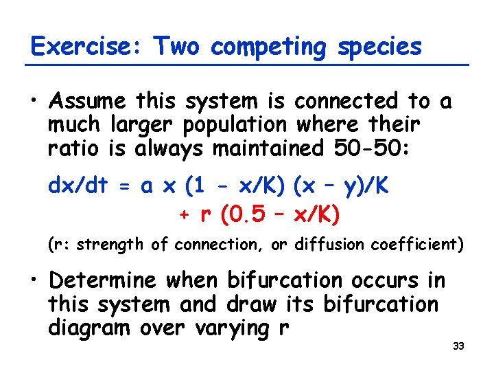
Exercise: Two competing species • Assume this system is connected to a much larger population where their ratio is always maintained 50 -50: dx/dt = a x (1 - x/K) (x – y)/K + r (0. 5 – x/K) (r: strength of connection, or diffusion coefficient) • Determine when bifurcation occurs in this system and draw its bifurcation diagram over varying r 33

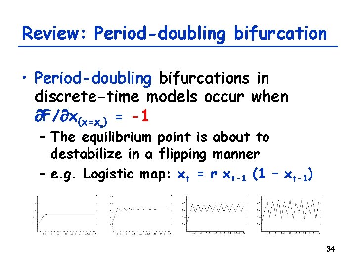
Review: Period-doubling bifurcation • Period-doubling bifurcations in discrete-time models occur when F/ x(x=xe) = -1 – The equilibrium point is about to destabilize in a flipping manner – e. g. Logistic map: xt = r xt-1 (1 – xt-1) 34

Limit Cycles and Hopf Bifurcations in Higher-Dimensional Systems 35

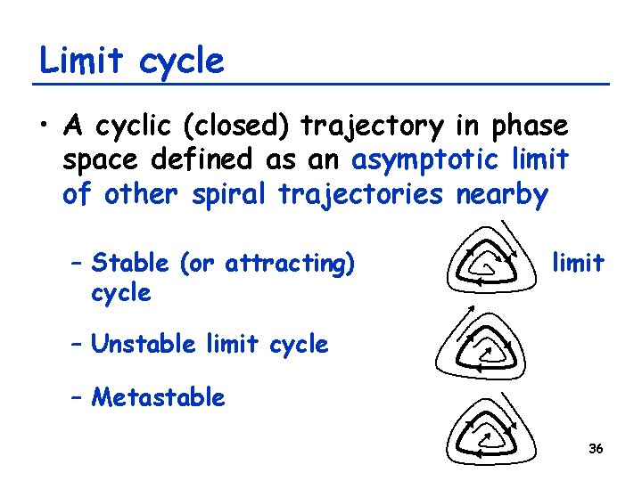
Limit cycle • A cyclic (closed) trajectory in phase space defined as an asymptotic limit of other spiral trajectories nearby – Stable (or attracting) cycle limit – Unstable limit cycle – Metastable 36

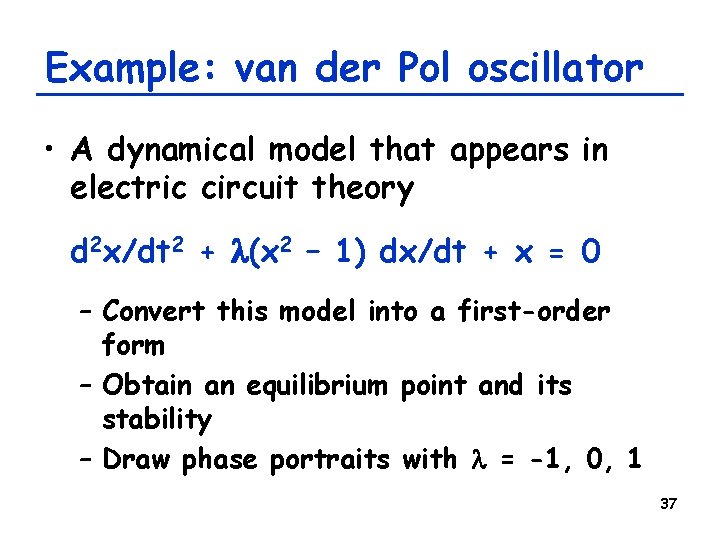
Example: van der Pol oscillator • A dynamical model that appears in electric circuit theory d 2 x/dt 2 + l(x 2 – 1) dx/dt + x = 0 – Convert this model into a first-order form – Obtain an equilibrium point and its stability – Draw phase portraits with l = -1, 0, 1 37

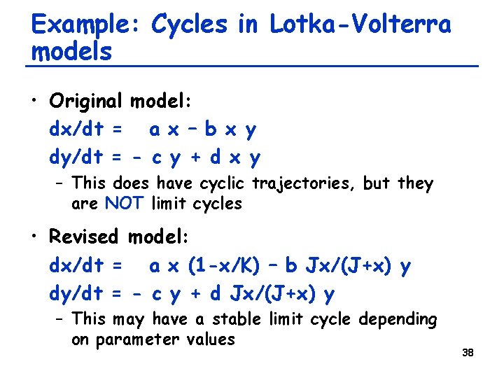
Example: Cycles in Lotka-Volterra models • Original model: dx/dt = a x – b x y dy/dt = - c y + d x y – This does have cyclic trajectories, but they are NOT limit cycles • Revised model: dx/dt = a x (1 -x/K) – b Jx/(J+x) y dy/dt = - c y + d Jx/(J+x) y – This may have a stable limit cycle depending on parameter values 38

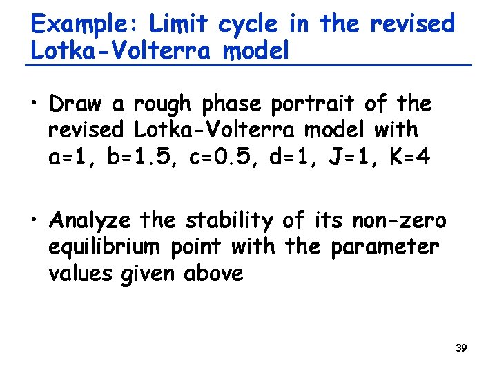
Example: Limit cycle in the revised Lotka-Volterra model • Draw a rough phase portrait of the revised Lotka-Volterra model with a=1, b=1. 5, c=0. 5, d=1, J=1, K=4 • Analyze the stability of its non-zero equilibrium point with the parameter values given above 39

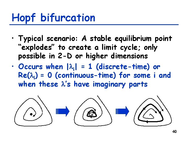
Hopf bifurcation • Typical scenario: A stable equilibrium point “explodes” to create a limit cycle; only possible in 2 -D or higher dimensions • Occurs when |li| = 1 (discrete-time) or Re(li) = 0 (continuous-time) for some i and when these l’s have imaginary parts 40

Exercise: Hopf-bifurcation in the revised Lotka-Volterra model • Analyze the stability of the non-zero equilibrium point of the revised Lotka. Volterra model with a=1, b=1. 5, c=0. 5, d=1, K=4, while leaving J as a variable (control parameter) • Figure out at what value of J the system undergoes Hopf bifurcation • Plot several phase portraits with varying J near its critical value 41

Hopf Bifurcations in Neuronal Models 42

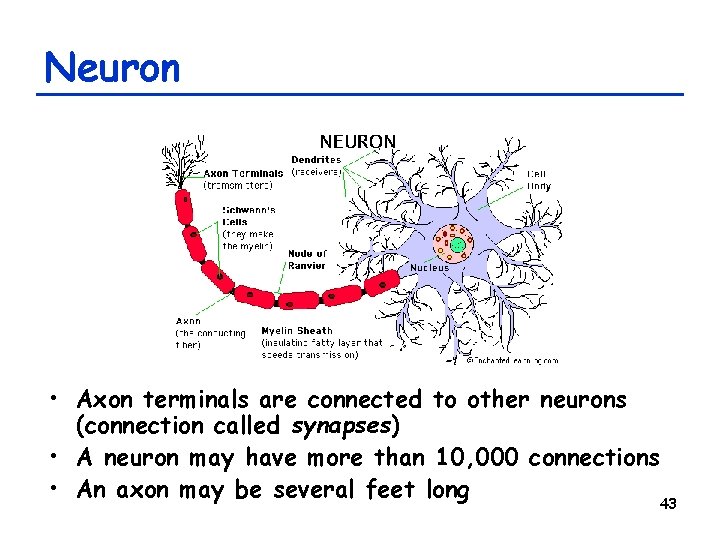
Neuron • Axon terminals are connected to other neurons (connection called synapses) • A neuron may have more than 10, 000 connections • An axon may be several feet long 43

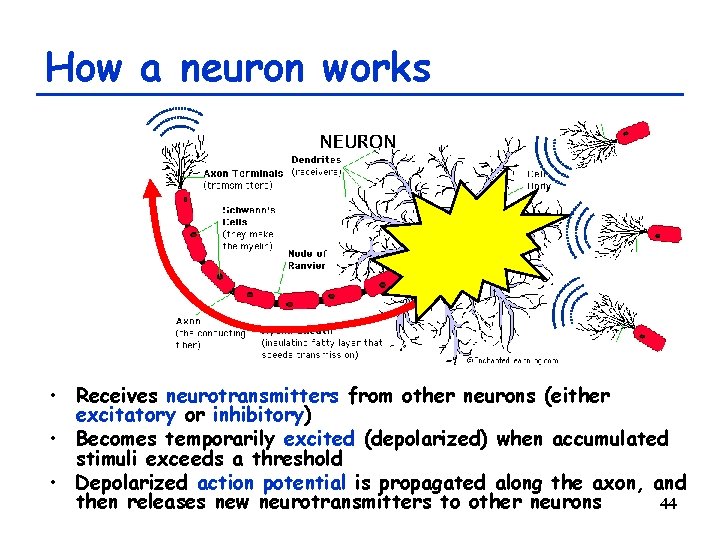
How a neuron works • Receives neurotransmitters from other neurons (either excitatory or inhibitory) • Becomes temporarily excited (depolarized) when accumulated stimuli exceeds a threshold • Depolarized action potential is propagated along the axon, and then releases new neurotransmitters to other neurons 44

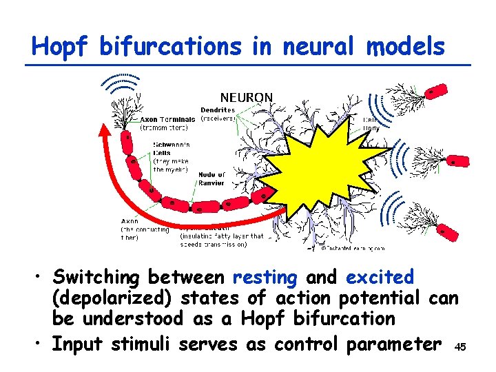
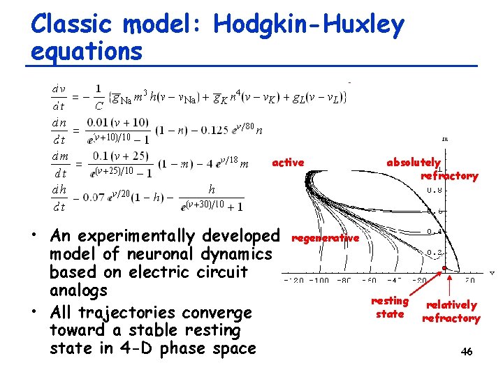
Hopf bifurcations in neural models • Switching between resting and excited (depolarized) states of action potential can be understood as a Hopf bifurcation • Input stimuli serves as control parameter 45

Classic model: Hodgkin-Huxley equations active • An experimentally developed model of neuronal dynamics based on electric circuit analogs • All trajectories converge toward a stable resting state in 4 -D phase space absolutely refractory regenerative resting state relatively refractory 46

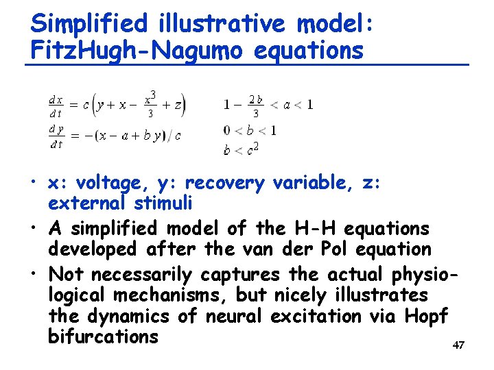
Simplified illustrative model: Fitz. Hugh-Nagumo equations • x: voltage, y: recovery variable, z: external stimuli • A simplified model of the H-H equations developed after the van der Pol equation • Not necessarily captures the actual physiological mechanisms, but nicely illustrates the dynamics of neural excitation via Hopf bifurcations 47

Exercise • Assume a=0. 7, b=0. 8 and c=3 • Obtain analytically the equilibrium point of the F-N equations (there is only one real equilibrium point) • Evaluate the stability of that point • Identify when Hopf bifurcation occurs 48

Chaos in Continuous-Time Models 49

Chaos in continuous-time models • Requires three or more dimensions – Because in 1 -D or 2 -D phase space, every trajectory works as a “wall” and thus confines where you can go in the future; stretching and folding are not possible in such an environment TRON / © Walt Disney Pictures 50

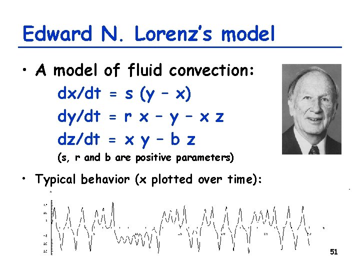
Edward N. Lorenz’s model • A model of fluid convection: dx/dt = s (y – x) dy/dt = r x – y – x z dz/dt = x y – b z (s, r and b are positive parameters) • Typical behavior (x plotted over time): 51

Exercise • Obtain the equilibrium points of the Lorenz model as a function of r while keeping s = 10 and b = 8/3 • Examine their stability and its dependence on the value of r • When do bifurcations occur? 52

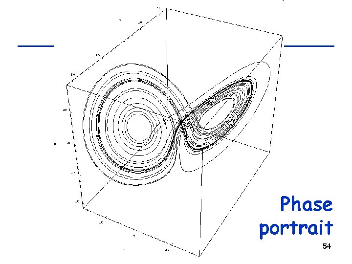
Exercise • Draw phase portraits of the Lorenz model by either projecting it to a 2 -D space or plotting in a 3 -D space – Not to mess up the plot, it is suggested that you plot only one sample trajectory starting from a single initial condition • Try several different values of r and see what you will get 53

Phase portrait 54

Strange attractor • A bounded region in a phase space that attracts nearby trajectories but also exhibits sensitive dependence on initial conditions inside it (i. e. , no convergence to fixed points or periodic trajectories) – A. k. a. : chaotic attractor, fractal attractor 55

Exercise: Finding stretch and folding in the Lorenz model • Interpret the structure of the strange attractor of the Lorenz model and find how “stretch and folding” of phase space is achieved 56

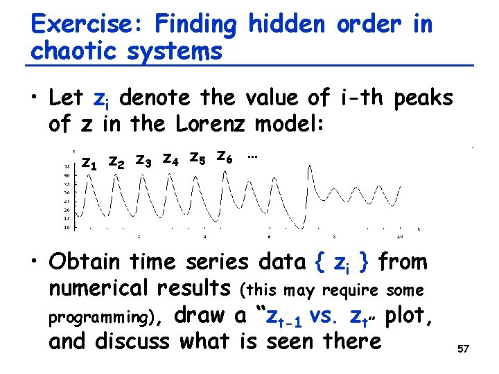
Exercise: Finding hidden order in chaotic systems • Let zi denote the value of i-th peaks of z in the Lorenz model: z 1 z 2 z 3 z 4 z 5 z 6 … • Obtain time series data { zi } from numerical results (this may require some programming), draw a “zt-1 vs. zt” plot, and discuss what is seen there 57

Mean-Field Approximation (will be revisited later) 58

Limitations of phase space-based approaches • Phase space visualization is impossible for high-dimensional systems – E. g. models with 20 variables, either continuous or discrete • Some phase space analysis techniques works for continuous models only – E. g. linear stability analysis does not work for discrete-state models where infinitely small noise cannot be assumed 59

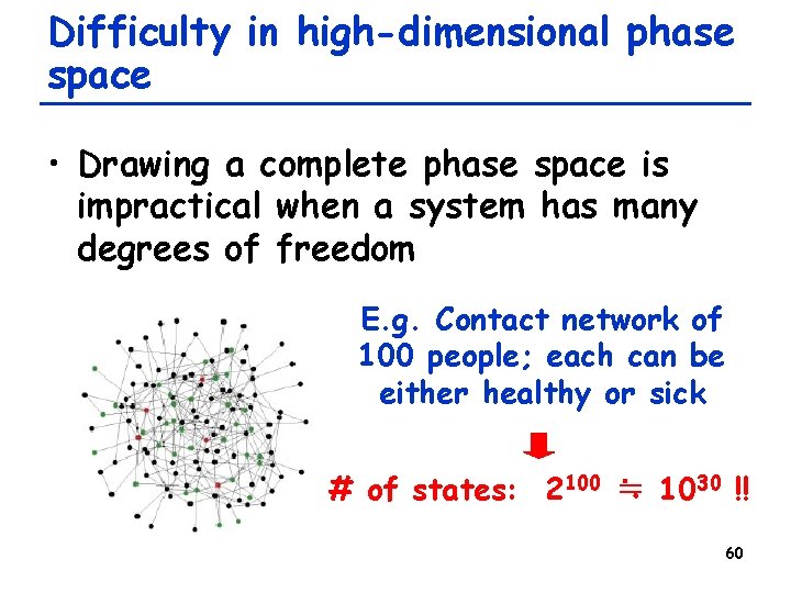
Difficulty in high-dimensional phase space • Drawing a complete phase space is impractical when a system has many degrees of freedom E. g. Contact network of 100 people; each can be either healthy or sick # of states: 2100 ≒ 1030 !! 60

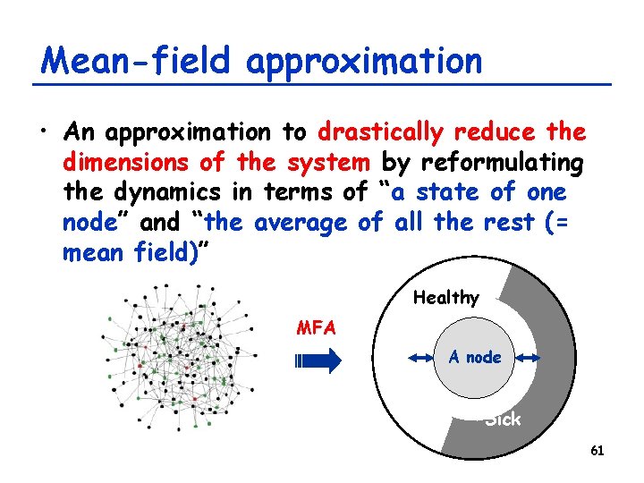
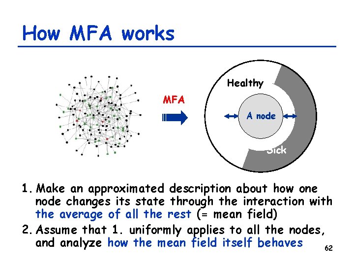
Mean-field approximation • An approximation to drastically reduce the dimensions of the system by reformulating the dynamics in terms of “a state of one node” and “the average of all the rest (= mean field)” Healthy MFA A node Sick 61

How MFA works Healthy MFA A node Sick 1. Make an approximated description about how one node changes its state through the interaction with the average of all the rest (= mean field) 2. Assume that 1. uniformly applies to all the nodes, and analyze how the mean field itself behaves 62

Mathematical description of MFA (difference equations) • Original equations: xit = Fi( { xit-1 } ) • Approximate equations with MFA: xit = F’i(xit-1, <x>t-1) <x>t = Si xit-1 / n Each state-transition function takes only two arguments: its own state and the “mean field” 63

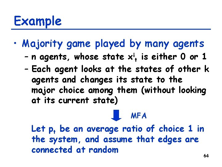
Example • Majority game played by many agents – n agents, whose state xit is either 0 or 1 – Each agent looks at the states of other k agents and changes its state to the major choice among them (without looking at its current state) MFA Let pt be an average ratio of choice 1 in the system, and assume that edges are connected at random 64

Exercise • Describe the probability for choice 1 to be a majority among the k other agents using pt • Write down a MFA version of the state-transition equations • Consider how the mean field pt changes along time 65

Answer • Probability for choice 1 to be a majority among the k other agents: rt = Sk/2<m<=k m (1 -p )k-m C p k m t t • State-transition equations: x it = 1 (with prob. rt-1) or 0 (otherwise) • Change of the mean field pt: pt = Si xit / n = rt-1 (if n is large) = Sk/2<m<=k k. Cm pt-1 m (1 -pt-1)k-m 66

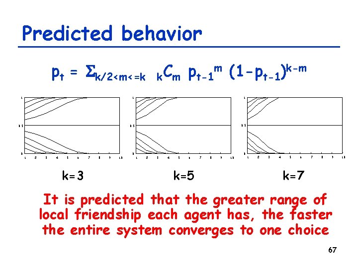
Predicted behavior pt = Sk/2<m<=k m (1 -p k-m C p ) k m t-1 1 1 1 0. 5 0 1 2 3 4 5 6 k=3 7 8 9 10 0 1 2 3 4 5 6 k=5 7 8 9 10 0 1 2 3 4 5 6 7 8 9 k=7 It is predicted that the greater range of local friendship each agent has, the faster the entire system converges to one choice 67 10

Exercise • Consider the propagation of flu over a large social network in which people are randomly connected to others • A pair of people are connected with each other at small probability p • Flu infects from an infected person to her susceptible neighbors at 100% probability • An infected person will immediately come back to susceptible at next time step thanks to medication (but no immunity acquired; SIS model) 68

Exercise • Assume there are n people in total, and there is only one infected person at the beginning • Describe how the ratio of infected people changes over time using MFA – What is the critical value of p? – State of each person: { 0, 1 } (0: susceptible, 1: infected) – Mean field variable: rt (Ratio of infected people within society) 69

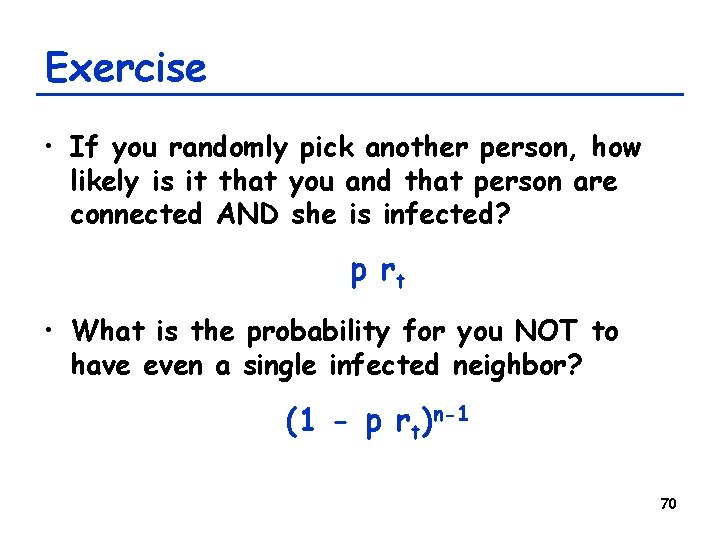
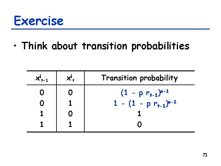
Exercise • If you randomly pick another person, how likely is it that you and that person are connected AND she is infected? p rt • What is the probability for you NOT to have even a single infected neighbor? (1 - p rt)n-1 70

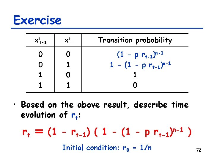
Exercise • Think about transition probabilities xit-1 x it Transition probability 0 0 1 1 0 1 (1 - p rt-1)n-1 1 - (1 - p rt-1)n-1 1 0 71

Exercise xit-1 x it Transition probability 0 0 1 1 0 1 (1 - p rt-1)n-1 1 - (1 - p rt-1)n-1 1 0 • Based on the above result, describe time evolution of rt: rt ＝ (1 - rt-1) ( 1 - (1 - p rt-1)n-1 ) Initial condition: r 0 = 1/n 72

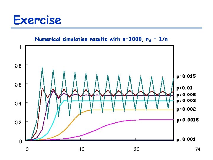
Exercise • What is the critical connection probability pc? – With pc, r stays its initial value (r 0) r 0 = (1 - r 0) ( 1 - (1 - pc r 0)n-1 ) – As pc r 0 is small, we may write: r 0 ~ (1 - r 0) ( 1 - (n - 1) pc r 0) ) pc ~ 1 / (1 - r 0) (n - 1) = n / (n - 1)2 73

Exercise Numerical simulation results with n=1000, r 0 = 1/n 1 0. 8 p=0. 015 0. 6 p=0. 01 p=0. 005 p=0. 003 0. 4 p=0. 002 p=0. 0015 0. 2 p=0. 001 0 0 10 20 74

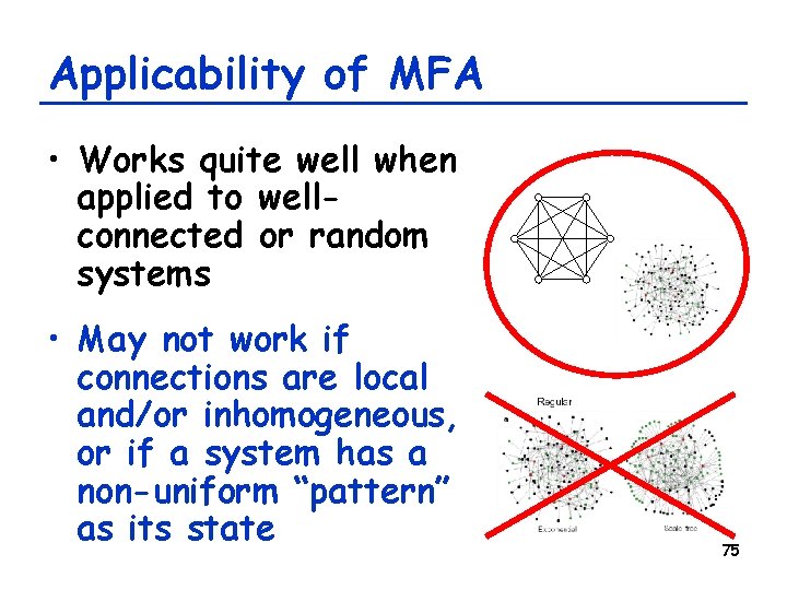
Applicability of MFA • Works quite well when applied to wellconnected or random systems • May not work if connections are local and/or inhomogeneous, or if a system has a non-uniform “pattern” as its state 75

Summary • To study the dynamics of nonlinear systems, there are several analytical tools available: – Linear stability analysis – Bifurcation analysis – Mean-field approximation 76