NECSI Summer School 2008 Week 3 Methods for

NECSI Summer School 2008 Week 3: Methods for the Study of Complex Systems Cellular Automata Hiroki Sayama sayama@binghamton. edu

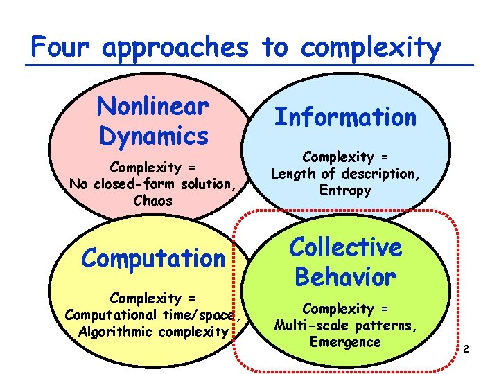
Four approaches to complexity Nonlinear Dynamics Complexity = No closed-form solution, Chaos Computation Complexity = Computational time/space, Algorithmic complexity Information Complexity = Length of description, Entropy Collective Behavior Complexity = Multi-scale patterns, Emergence 2

Review of Cellular Automata 3

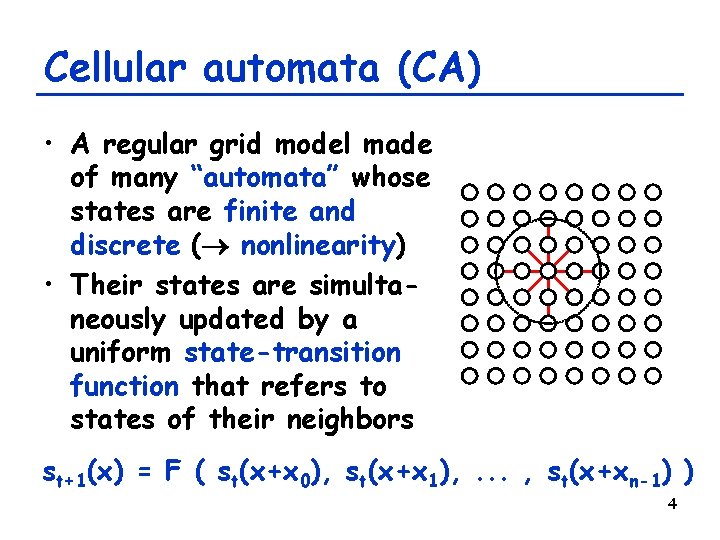
Cellular automata (CA) • A regular grid model made of many “automata” whose states are finite and discrete ( nonlinearity) • Their states are simultaneously updated by a uniform state-transition function that refers to states of their neighbors st+1(x) = F ( st(x+x 0), st(x+x 1), . . . , st(x+xn-1) ) 4

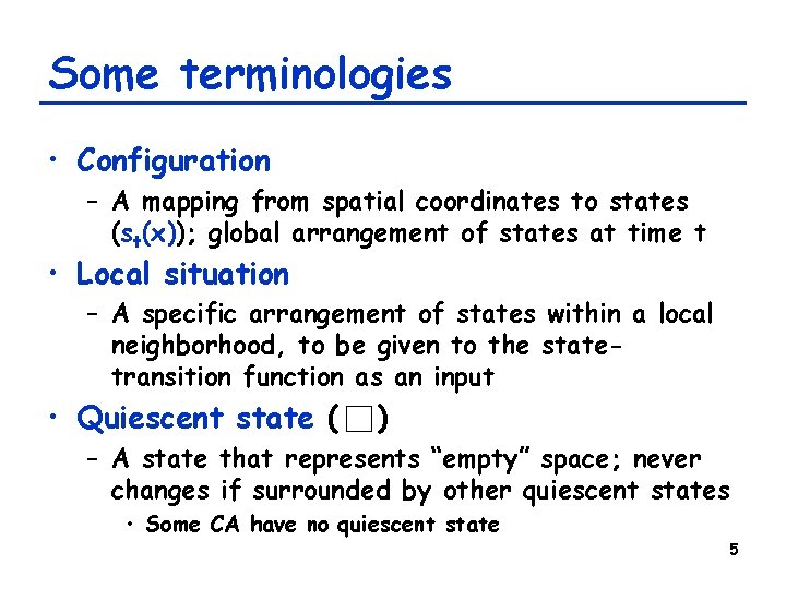
Some terminologies • Configuration – A mapping from spatial coordinates to states (st(x)); global arrangement of states at time t • Local situation – A specific arrangement of states within a local neighborhood, to be given to the statetransition function as an input • Quiescent state ( ) – A state that represents “empty” space; never changes if surrounded by other quiescent states • Some CA have no quiescent state 5

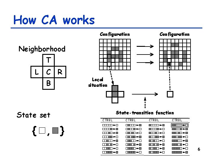
How CA works Configuration Neighborhood T L C R B State set Local situation State-transition function CTRBL { , } 6

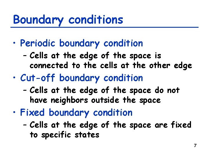
Boundary conditions • Periodic boundary condition – Cells at the edge of the space is connected to the cells at the other edge • Cut-off boundary condition – Cells at the edge of the space do not have neighbors outside the space • Fixed boundary condition – Cells at the edge of the space are fixed to specific states 7

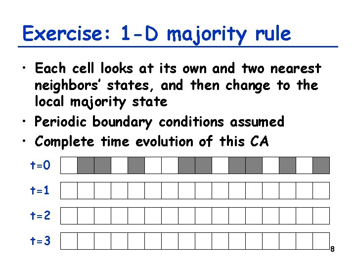
Exercise: 1 -D majority rule • Each cell looks at its own and two nearest neighbors’ states, and then change to the local majority state • Periodic boundary conditions assumed • Complete time evolution of this CA t=0 t=1 t=2 t=3 8

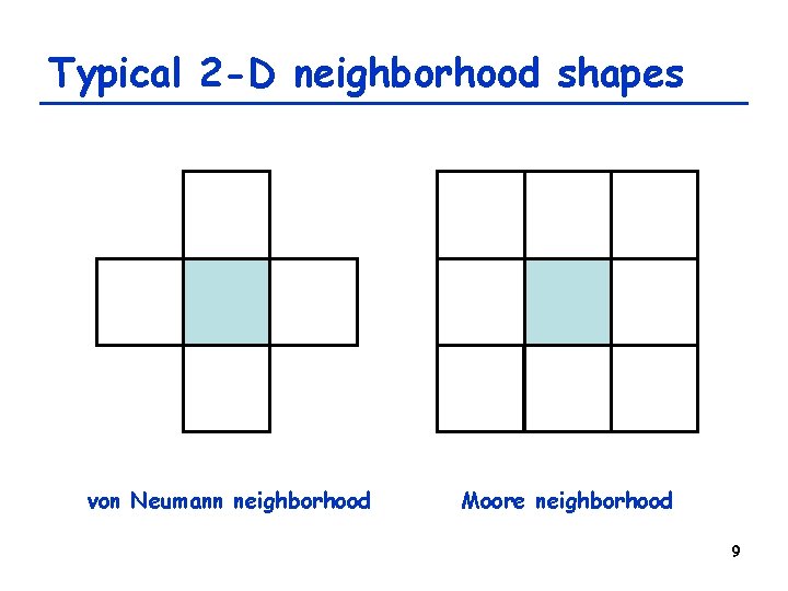
Typical 2 -D neighborhood shapes von Neumann neighborhood Moore neighborhood 9

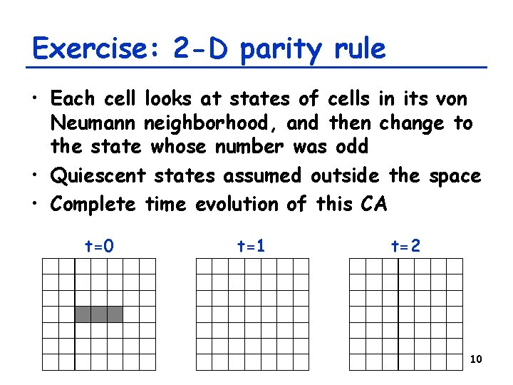
Exercise: 2 -D parity rule • Each cell looks at states of cells in its von Neumann neighborhood, and then change to the state whose number was odd • Quiescent states assumed outside the space • Complete time evolution of this CA t=0 t=1 t=2 10

Phase Space of Cellular Automata 11

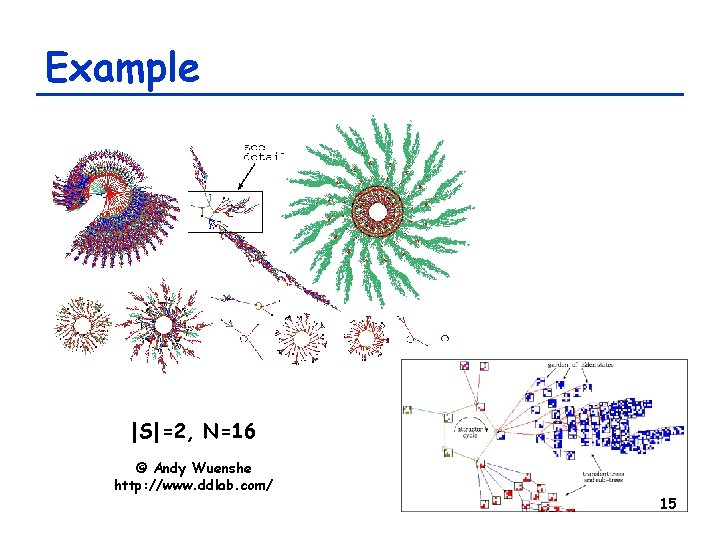
Phase space of cellular automata • For a fixed number of cells, the total number of possible configurations is also fixed and finite: |S|N – S: State set – N: Total number of cells • For deterministic CA, each configuration is always mapped to just one configuration – You can draw a state-transition diagram 12

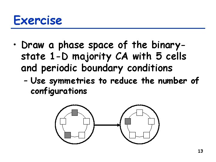
Exercise • Draw a phase space of the binarystate 1 -D majority CA with 5 cells and periodic boundary conditions – Use symmetries to reduce the number of configurations 13

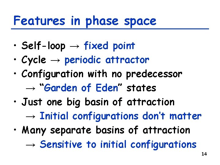
Features in phase space • Self-loop → fixed point • Cycle → periodic attractor • Configuration with no predecessor → “Garden of Eden” states • Just one big basin of attraction → Initial configurations don’t matter • Many separate basins of attraction → Sensitive to initial configurations 14

Example |S|=2, N=16 © Andy Wuenshe http: //www. ddlab. com/ 15

Wolfram’s classification • Wolfram (1984) classified binarystate 1 -D CA based on their typical attractors’ properties – I: Fixed point of homogeneous states – II: Fixed point or small cycle involving heterogeneous states – III: Chaotic attractor (very long cycle) – IV: Complex, long-lived localized structures (attractor preceded by very long tree-like basins of attraction) 16

Wolfram’s classification 17

Reversible CA • Some CA rules are reversible – Every configuration has one and only one predecessor configuration – May or may not be locally reversible • Reversible CA has a particular type of phase space – There are only cycles or fixed points; no trees, branches – All the fixed points are isolated 18

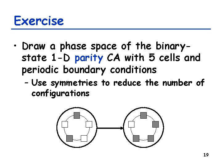
Exercise • Draw a phase space of the binarystate 1 -D parity CA with 5 cells and periodic boundary conditions – Use symmetries to reduce the number of configurations 19

Converting PDE Models into CA with Real-Valued States 20

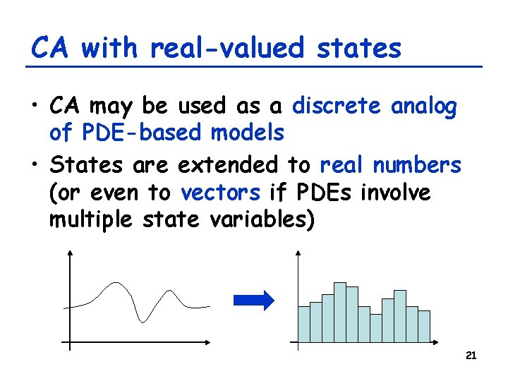
CA with real-valued states • CA may be used as a discrete analog of PDE-based models • States are extended to real numbers (or even to vectors if PDEs involve multiple state variables) 21

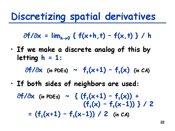
Discretizing spatial derivatives f/ x = limh 0 { f(x+h, t) – f(x, t) } / h • If we make a discrete analog of this by letting h = 1: f/ x (in PDEs) ~ ft(x+1) – ft(x) (in CA) • If both sides of neighbors are used: ~ { (ft(x+1) – ft(x)) + (ft(x) – ft(x-1)) } / 2 = (ft(x+1) – ft(x-1)) / 2 (in CA) f/ x (in PDEs) 22

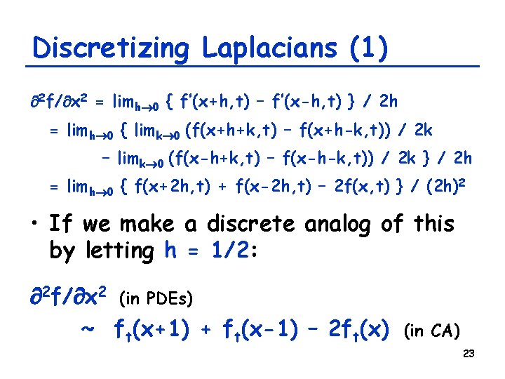
Discretizing Laplacians (1) 2 f/ x 2 = limh 0 { f’(x+h, t) – f’(x-h, t) } / 2 h = limh 0 { limk 0 (f(x+h+k, t) – f(x+h-k, t)) / 2 k – limk 0 (f(x-h+k, t) – f(x-h-k, t)) / 2 k } / 2 h = limh 0 { f(x+2 h, t) + f(x-2 h, t) – 2 f(x, t) } / (2 h)2 • If we make a discrete analog of this by letting h = 1/2: 2 f/ x 2 (in PDEs) ~ ft(x+1) + ft(x-1) – 2 ft(x) (in CA) 23

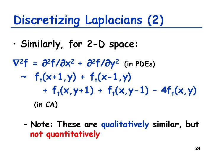
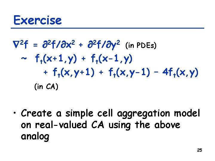
Discretizing Laplacians (2) • Similarly, for 2 -D space: 2 f = 2 f/ x 2 + 2 f/ y 2 (in PDEs) ~ ft(x+1, y) + ft(x-1, y) + ft(x, y+1) + ft(x, y-1) – 4 ft(x, y) (in CA) – Note: These are qualitatively similar, but not quantitatively 24

Exercise 2 f = 2 f/ x 2 + 2 f/ y 2 (in PDEs) ~ ft(x+1, y) + ft(x-1, y) + ft(x, y+1) + ft(x, y-1) – 4 ft(x, y) (in CA) • Create a simple cell aggregation model on real-valued CA using the above analog 25

Other Extensions of Cellular Automata 26

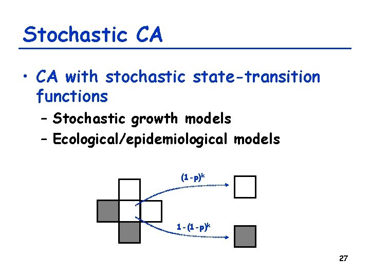
Stochastic CA • CA with stochastic state-transition functions – Stochastic growth models – Ecological/epidemiological models (1 -p)k 1 -(1 -p)k 27

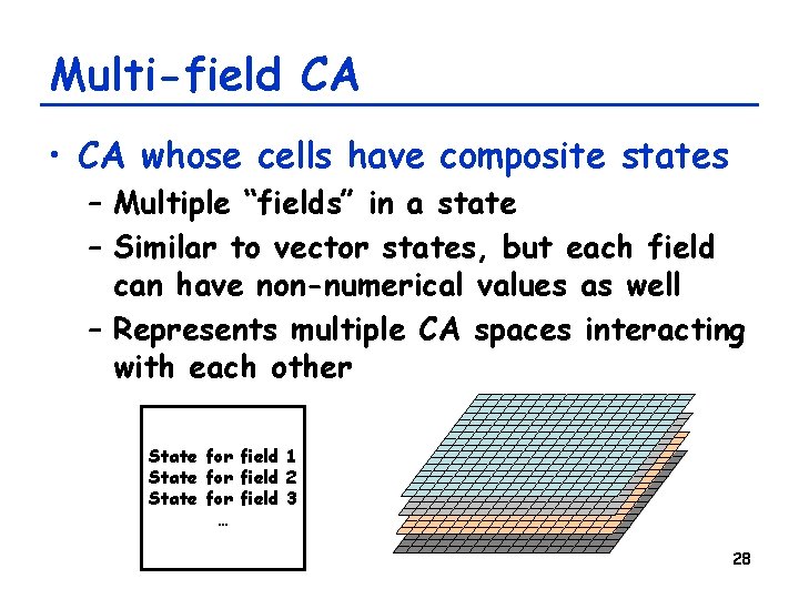
Multi-field CA • CA whose cells have composite states – Multiple “fields” in a state – Similar to vector states, but each field can have non-numerical values as well – Represents multiple CA spaces interacting with each other State for field 1 State for field 2 State for field 3 … 28

Multi-field CA • Examples – Models of spatially distributed agents with complex internal states – Models of interaction between agents and environment – CA that depend on more than one step past configurations 29

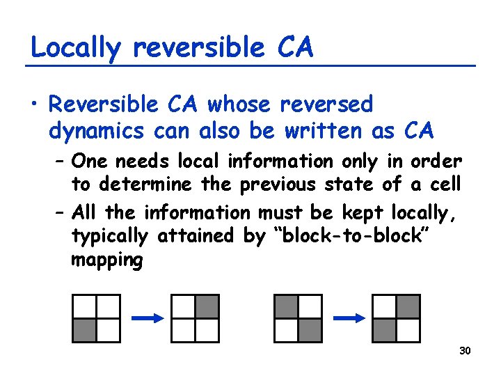
Locally reversible CA • Reversible CA whose reversed dynamics can also be written as CA – One needs local information only in order to determine the previous state of a cell – All the information must be kept locally, typically attained by “block-to-block” mapping 30

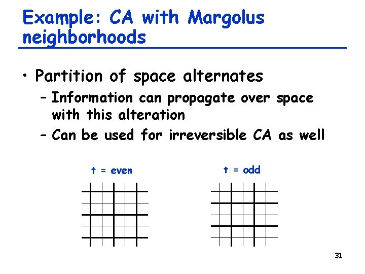
Example: CA with Margolus neighborhoods • Partition of space alternates – Information can propagate over space with this alteration – Can be used for irreversible CA as well t = even t = odd 31

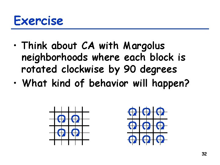
Exercise • Think about CA with Margolus neighborhoods where each block is rotated clockwise by 90 degrees • What kind of behavior will happen? 32

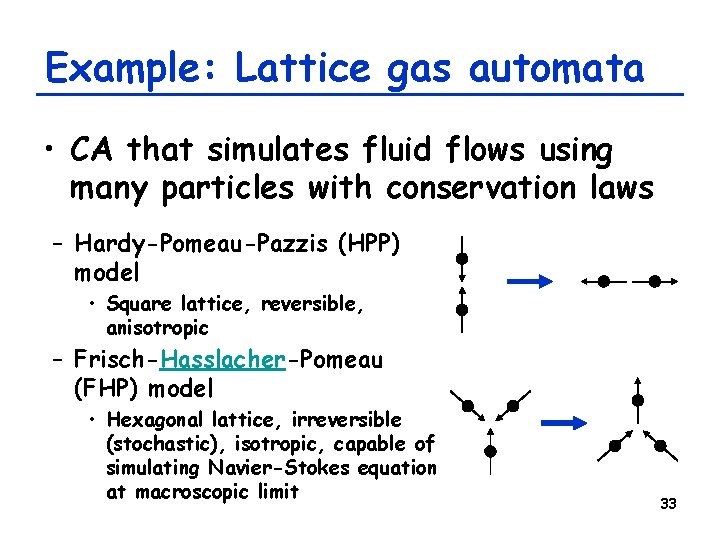
Example: Lattice gas automata • CA that simulates fluid flows using many particles with conservation laws – Hardy-Pomeau-Pazzis (HPP) model • Square lattice, reversible, anisotropic – Frisch-Hasslacher-Pomeau (FHP) model • Hexagonal lattice, irreversible (stochastic), isotropic, capable of simulating Navier-Stokes equation at macroscopic limit 33

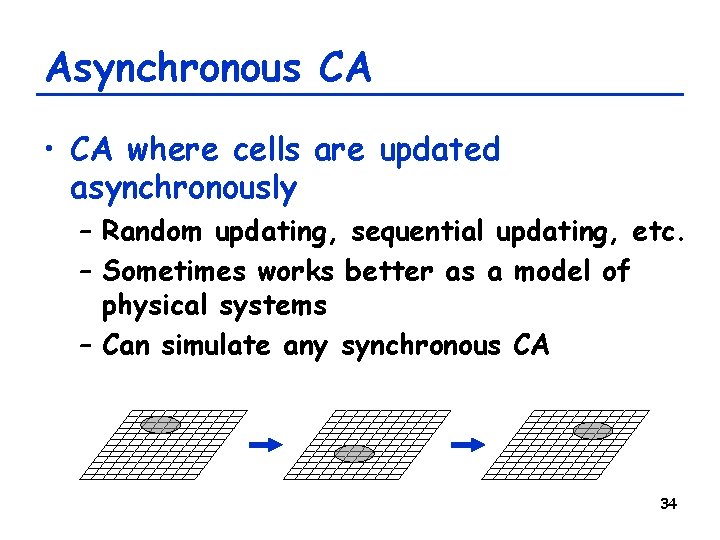
Asynchronous CA • CA where cells are updated asynchronously – Random updating, sequential updating, etc. – Sometimes works better as a model of physical systems – Can simulate any synchronous CA 34

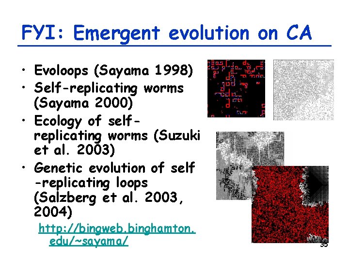
FYI: Emergent evolution on CA • Evoloops (Sayama 1998) • Self-replicating worms (Sayama 2000) • Ecology of selfreplicating worms (Suzuki et al. 2003) • Genetic evolution of self -replicating loops (Salzberg et al. 2003, 2004) http: //bingweb. binghamton. edu/~sayama/ 35

Summary • Cellular automata are extensively used for complex systems modeling • Phase space structure of CA determines their dynamical properties • CA may be used as a substitute for PDE-based models • Several non-traditional model extensions are possible 36