NECSI Summer School 2008 Week 3 Methods for

NECSI Summer School 2008 Week 3: Methods for the Study of Complex Systems Partial Differential Equations and Reaction-Diffusion Systems Hiroki Sayama sayama@binghamton. edu

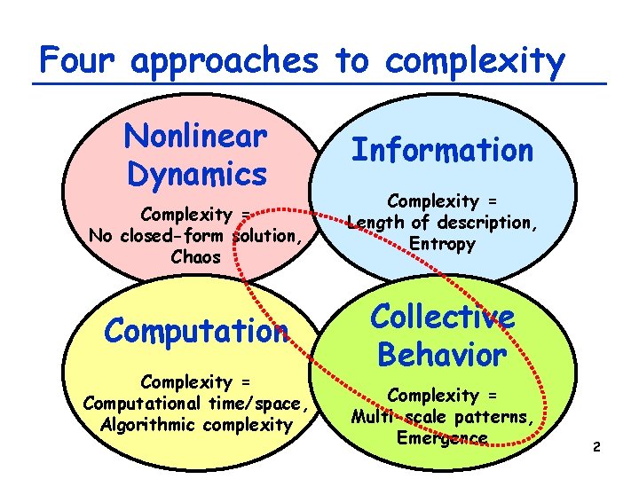
Four approaches to complexity Nonlinear Dynamics Complexity = No closed-form solution, Chaos Computation Complexity = Computational time/space, Algorithmic complexity Information Complexity = Length of description, Entropy Collective Behavior Complexity = Multi-scale patterns, Emergence 2

Continuous Field Models 3

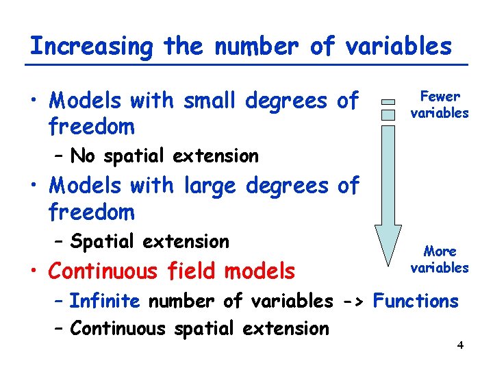
Increasing the number of variables • Models with small degrees of freedom Fewer variables – No spatial extension • Models with large degrees of freedom – Spatial extension • Continuous field models More variables – Infinite number of variables -> Functions – Continuous spatial extension 4

Continuous field models • A system’s state is represented by a function that maps each spatial location to a local state value/vector • Dynamics are described typically using partial differential equations (PDEs) • Analytical treatments may still be possible; may give us important solutions and insights 5

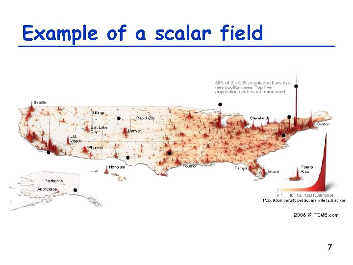
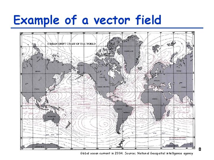
Spatial function as a “state” • The state of a PDE-based system is defined by a function f(x, t) – A field made of local states defined over a continuous spatial domain • x: spatial location (vector) • f(x, t): local state (scalar or vector) – Population density (scalar) – Chemical concentration (scalar or vector) – Local flow (vector) 6

Example of a scalar field 2006 © TIME. com 7

Example of a vector field Global ocean current in 2004. Source: National Geospatial intelligence agency 8

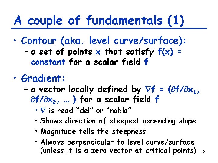
A couple of fundamentals (1) • Contour (aka. level curve/surface): – a set of points x that satisfy f(x) = constant for a scalar field f • Gradient: – a vector locally defined by f = ( f/ x 1, f/ x 2, … ) for a scalar field f • • is read “del” or “nabla” Shows direction of steepest ascending slope Magnitude tells the steepness Always perpendicular to level curve/surface (unless it is a zero vector at critical points) 9

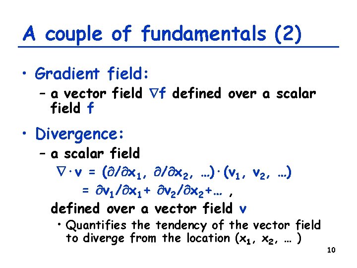
A couple of fundamentals (2) • Gradient field: – a vector field f defined over a scalar field f • Divergence: – a scalar field ·v = ( / x 1, / x 2, …)·(v 1, v 2, …) = v 1/ x 1+ v 2/ x 2+… , defined over a vector field v • Quantifies the tendency of the vector field to diverge from the location (x 1, x 2, … ) 10

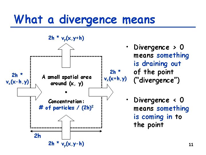
What a divergence means 2 h * vy(x, y+h) 2 h * vx(x-h, y) A small spatial area around (x, y) Concentration: # of particles / (2 h)2 • Divergence > 0 means something is draining out 2 h * of the point vx(x+h, y) (“divergence”) • Divergence < 0 means something is coming in to the point 2 h 2 h * vy(x, y-h) 11

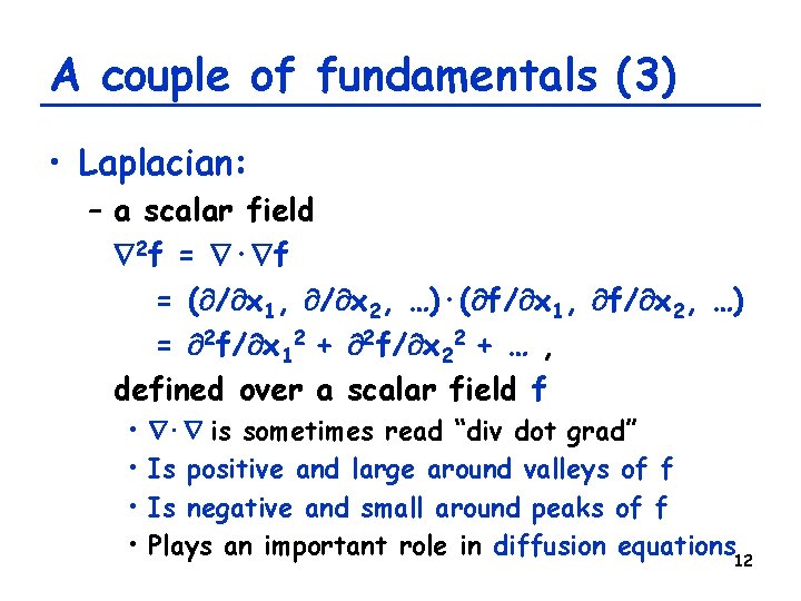
A couple of fundamentals (3) • Laplacian: – a scalar field 2 f = · f = ( / x 1, / x 2, …)·( f/ x 1, f/ x 2, …) = 2 f/ x 12 + 2 f/ x 22 + … , defined over a scalar field f • • · is sometimes read “div dot grad” Is positive and large around valleys of f Is negative and small around peaks of f Plays an important role in diffusion equations 12

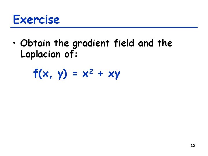
Exercise • Obtain the gradient field and the Laplacian of: f(x, y) = x 2 + xy 13

Developing PDE-Based Models 14

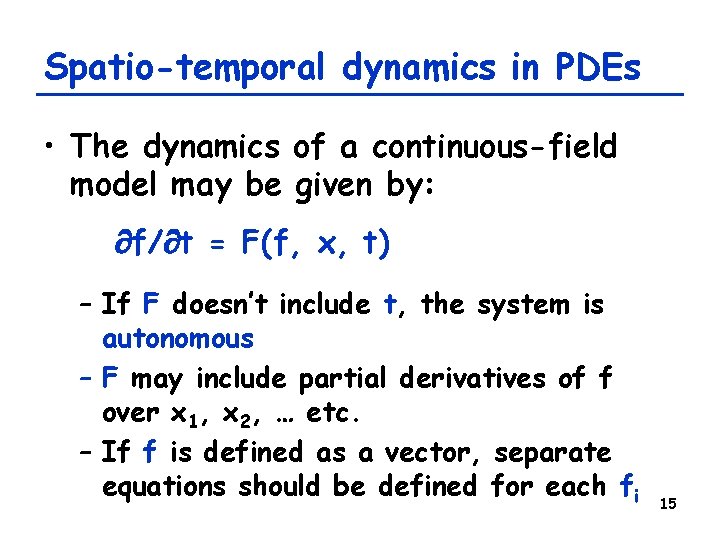
Spatio-temporal dynamics in PDEs • The dynamics of a continuous-field model may be given by: f/ t = F(f, x, t) – If F doesn’t include t, the system is autonomous – F may include partial derivatives of f over x 1, x 2, … etc. – If f is defined as a vector, separate equations should be defined for each fi 15

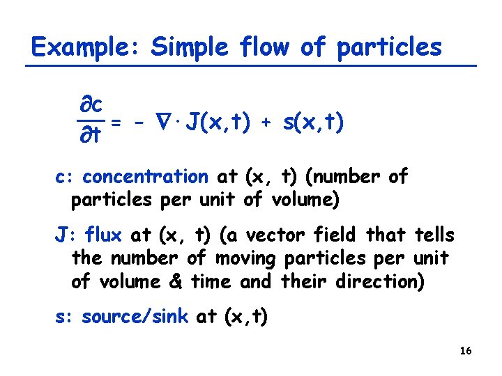
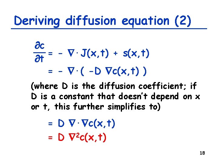
Example: Simple flow of particles c = - ·J(x, t) + s(x, t) t c: concentration at (x, t) (number of particles per unit of volume) J: flux at (x, t) (a vector field that tells the number of moving particles per unit of volume & time and their direction) s: source/sink at (x, t) 16

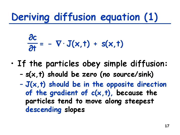
Deriving diffusion equation (1) c = - ·J(x, t) + s(x, t) t • If the particles obey simple diffusion: – s(x, t) should be zero (no source/sink) – J(x, t) should be in the opposite direction of the gradient of c(x, t), because the particles tend to move along steepest descending slopes 17

Deriving diffusion equation (2) c = - ·J(x, t) + s(x, t) t = - ·( -D c(x, t) ) (where D is the diffusion coefficient; if D is a constant that doesn’t depend on x or t, this further simplifies to) = D · c(x, t) = D 2 c(x, t) 18

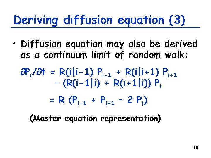
Deriving diffusion equation (3) • Diffusion equation may also be derived as a continuum limit of random walk: Pi/ t = R(i|i-1) Pi-1 + R(i|i+1) Pi+1 – (R(i-1|i) + R(i+1|i)) Pi = R (Pi-1 + Pi+1 – 2 Pi) (Master equation representation) 19

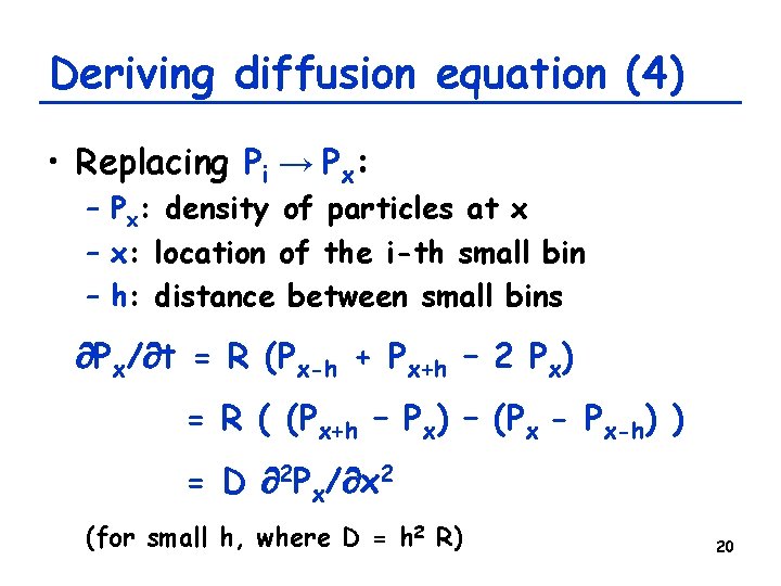
Deriving diffusion equation (4) • Replacing Pi → Px: – Px: density of particles at x – x: location of the i-th small bin – h: distance between small bins Px/ t = R (Px-h + Px+h – 2 Px) = R ( (Px+h – Px) – (Px - Px-h) ) = D 2 Px/ x 2 (for small h, where D = h 2 R) 20

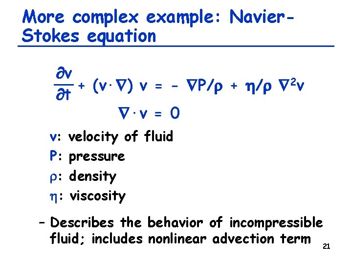
More complex example: Navier. Stokes equation v + (v· ) v = - P/r + h/r 2 v t ·v = 0 v: P: r: h: velocity of fluid pressure density viscosity – Describes the behavior of incompressible fluid; includes nonlinear advection term 21

Exercise • Develop a PDE model that describes the attraction of particles to each other – Assume each particle moves toward the regions where there are more particles 22

Exercise • Develop a two-variable PDE model that describes the spatio-temporal dynamics of the following system: – People are attracted toward the regions where economy is active – Economy is activated by having more people in the region – Economy would diminish without people – Both populations and economical activities diffuse spatially 23

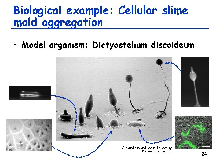
Biological example: Cellular slime mold aggregation • Model organism: Dictyostelium discoideum © dicty. Base and Kyoto University Dictyostelium Group 24

Model of slime mold aggregation • Developed by Keller & Segel (1970) • Assumptions: – Cells undergo random motion (diffusion) and chemotaxis toward c. AMP (attractant) – Cells neither die nor divide – Each cell constantly produce c. AMP – c. AMP shows diffusion and exponential decay • Note: Pretty much similar to the economy model we developed before!! 25

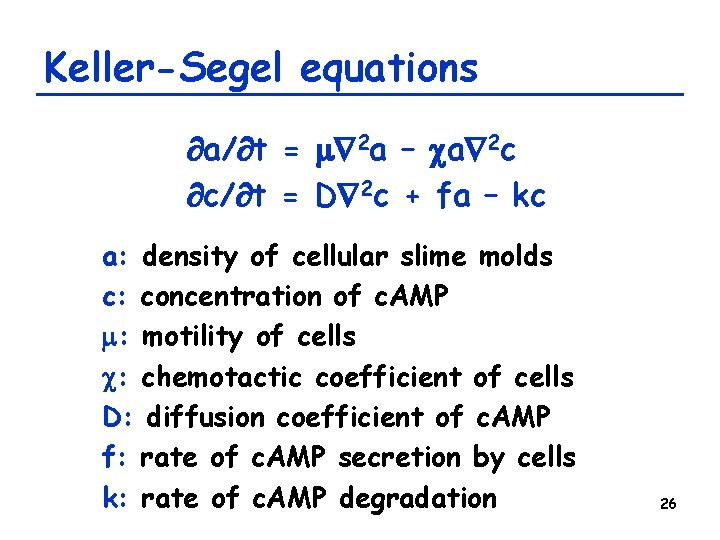
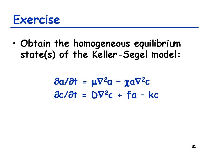
Keller-Segel equations a/ t = m 2 a – ca 2 c c/ t = D 2 c + fa – kc a: density of cellular slime molds c: concentration of c. AMP m: motility of cells c: chemotactic coefficient of cells D: diffusion coefficient of c. AMP f: rate of c. AMP secretion by cells k: rate of c. AMP degradation 26

Analytical Treatments of Spatially Distributed Systems 27

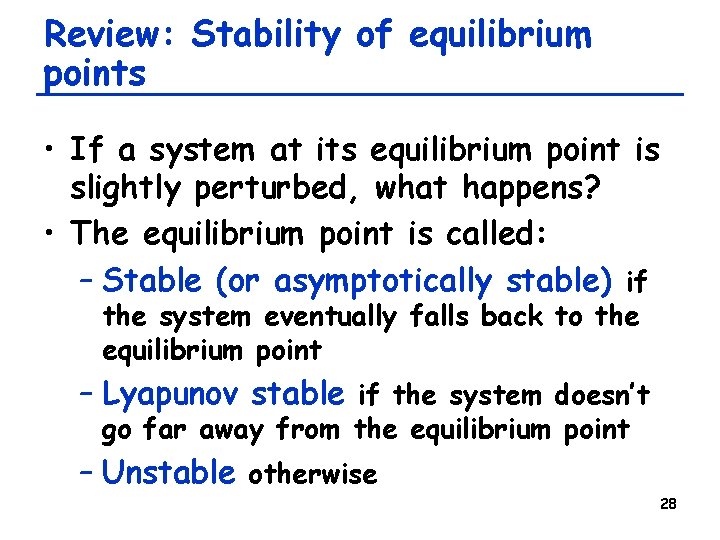
Review: Stability of equilibrium points • If a system at its equilibrium point is slightly perturbed, what happens? • The equilibrium point is called: – Stable (or asymptotically stable) if the system eventually falls back to the equilibrium point – Lyapunov stable if the system doesn’t go far away from the equilibrium point – Unstable otherwise 28

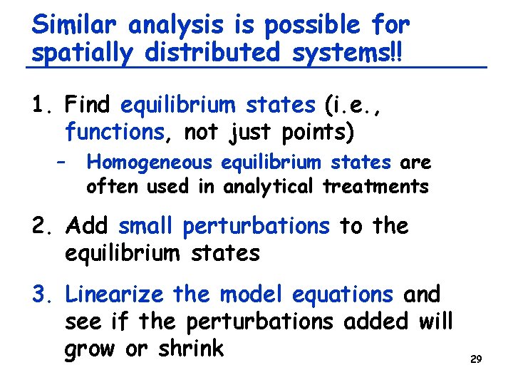
Similar analysis is possible for spatially distributed systems!! 1. Find equilibrium states (i. e. , functions, not just points) – Homogeneous equilibrium states are often used in analytical treatments 2. Add small perturbations to the equilibrium states 3. Linearize the model equations and see if the perturbations added will grow or shrink 29

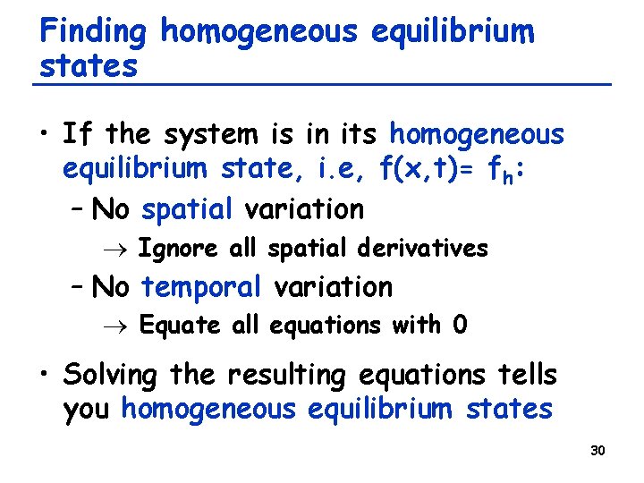
Finding homogeneous equilibrium states • If the system is in its homogeneous equilibrium state, i. e, f(x, t)= fh: – No spatial variation ® Ignore all spatial derivatives – No temporal variation ® Equate all equations with 0 • Solving the resulting equations tells you homogeneous equilibrium states 30

Exercise • Obtain the homogeneous equilibrium state(s) of the Keller-Segel model: a/ t = m 2 a – ca 2 c c/ t = D 2 c + fa – kc 31

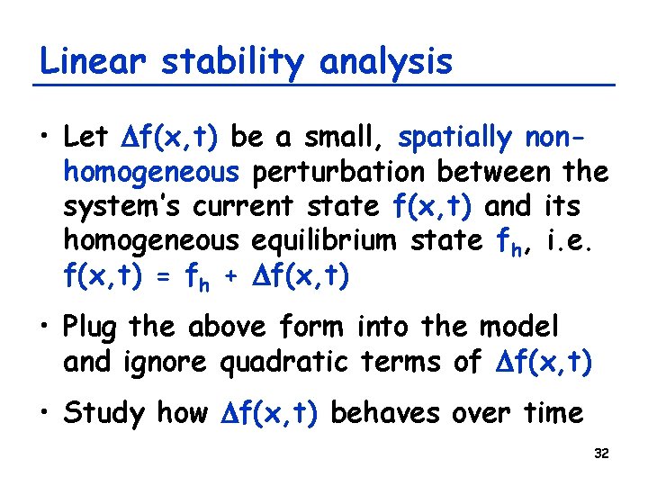
Linear stability analysis • Let Df(x, t) be a small, spatially nonhomogeneous perturbation between the system’s current state f(x, t) and its homogeneous equilibrium state fh, i. e. f(x, t) = fh + Df(x, t) • Plug the above form into the model and ignore quadratic terms of Df(x, t) • Study how Df(x, t) behaves over time 32

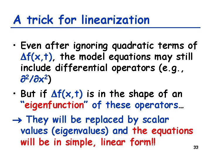
A trick for linearization • Even after ignoring quadratic terms of Df(x, t), the model equations may still include differential operators (e. g. , 2/ x 2) • But if Df(x, t) is in the shape of an “eigenfunction” of these operators… They will be replaced by scalar values (eigenvalues) and the equations will be in simple, linear form!! 33

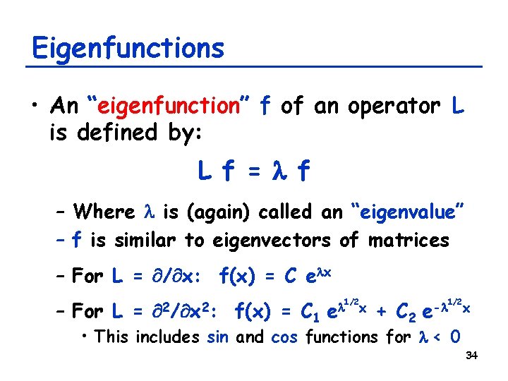
Eigenfunctions • An “eigenfunction” f of an operator L is defined by: L f = l f – Where l is (again) called an “eigenvalue” – f is similar to eigenvectors of matrices – For L = / x: f(x) = C elx – For L = 2/ x 2: f(x) = C 1 el 1/2 x + C 2 e-l 1/2 x • This includes sin and cos functions for l < 0 34

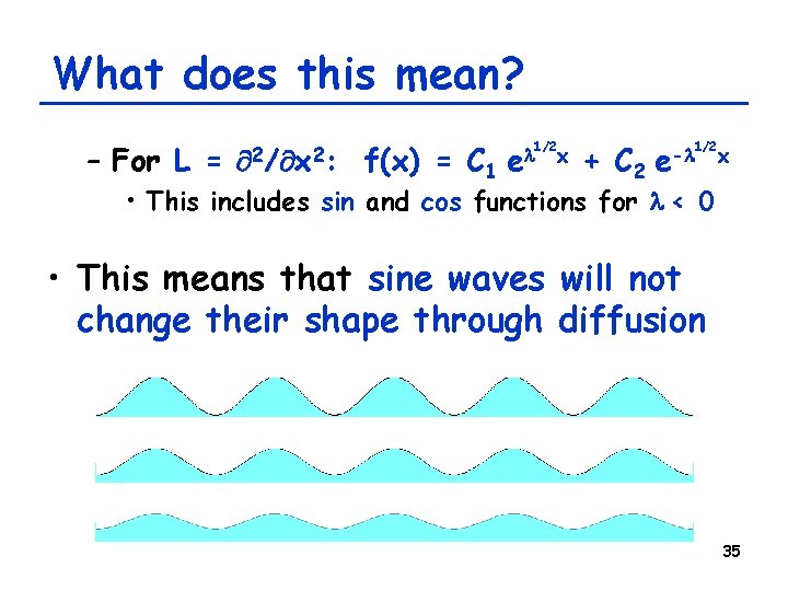
What does this mean? – For L = 2/ x 2: f(x) = C 1 el 1/2 x + C 2 e-l 1/2 x • This includes sin and cos functions for l < 0 • This means that sine waves will not change their shape through diffusion 35

Exercise • Sine waves will not change their shape through diffusion • Show the above fact mathematically in a 1 -D space – Let f(x, 0) = sin(qx+p) (initial condition) – Let f/ t = D 2 f (dynamics) – Solve the above equation and show that the solution is still the original sine wave 36

Linearizing model equations • For 1 -D diffusion-based models, the following perturbation is often used: Df(x, t) = Df(t) sin(qx+p) l l l Df(t): amplitude of small perturbation q: wavenumber (spatial frequency) p: phase offset (you may ignore this) 37

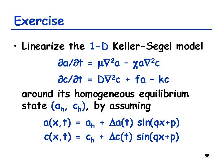
Exercise • Linearize the 1 -D Keller-Segel model a/ t = m 2 a – ca 2 c c/ t = D 2 c + fa – kc around its homogeneous equilibrium state (ah, ch), by assuming a(x, t) = ah + Da(t) sin(qx+p) c(x, t) = ch + Dc(t) sin(qx+p) 38

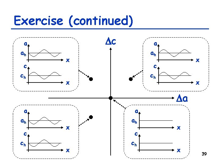
Exercise (continued) Dc a ah c ch a ah x x c ch x x Da a a ah ah c ch x x 39

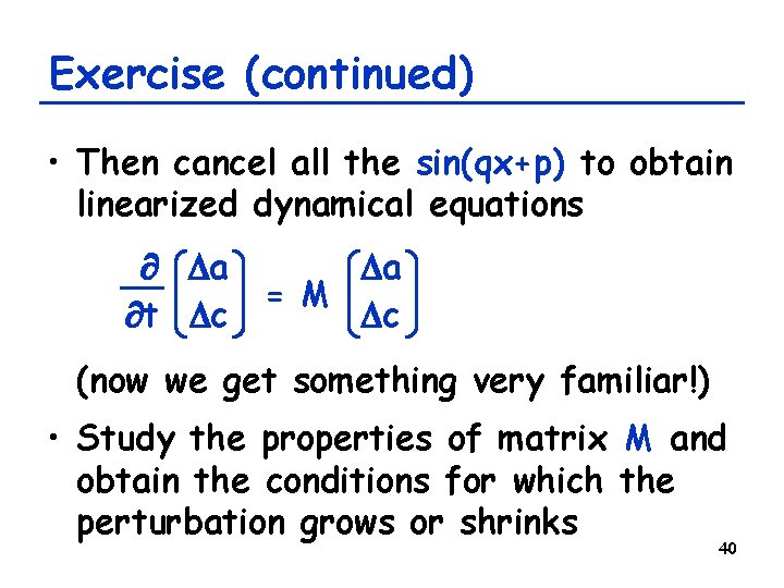
Exercise (continued) • Then cancel all the sin(qx+p) to obtain linearized dynamical equations Da t Dc Da = M Dc (now we get something very familiar!) • Study the properties of matrix M and obtain the conditions for which the perturbation grows or shrinks 40

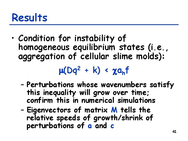
Results • Condition for instability of homogeneous equilibrium states (i. e. , aggregation of cellular slime molds): m(Dq 2 + k) < cahf – Perturbations whose wavenumbers satisfy this inequality will grow over time; confirm this in numerical simulations – Eigenvectors of matrix M tells the relative speeds of growth/shrink of perturbations of a and c 41

Reaction-Diffusion Equations 42

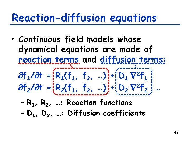
Reaction-diffusion equations • Continuous field models whose dynamical equations are made of reaction terms and diffusion terms: f 1/ t = R 1(f 1, f 2, …) + D 1 2 f 1 f 2/ t = R 2(f 1, f 2, …) + D 2 2 f 2 … – R 1, R 2, …: Reaction functions – D 1, D 2, …: Diffusion coefficients 43

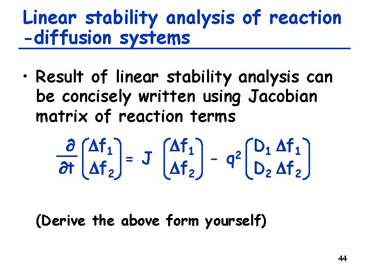
Linear stability analysis of reaction -diffusion systems • Result of linear stability analysis can be concisely written using Jacobian matrix of reaction terms Df 1 = J t Df 2 Df 1 D Df 1 1 2 - q Df 2 (Derive the above form yourself) 44

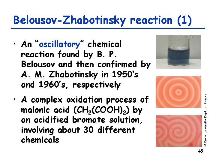
Belousov-Zhabotinsky reaction (1) • An “oscillatory” chemical reaction found by B. P. Belousov and then confirmed by A. M. Zhabotinsky in 1950‘s and 1960’s, respectively © Kyoto University Dept. of Physics • A complex oxidation process of malonic acid (CH 2(COOH)2) by an acidified bromate solution, involving about 30 different chemicals 45

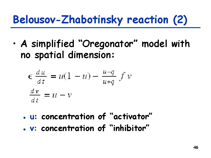
Belousov-Zhabotinsky reaction (2) • A simplified “Oregonator” model with no spatial dimension: l l u: concentration of “activator” v: concentration of “inhibitor” 46

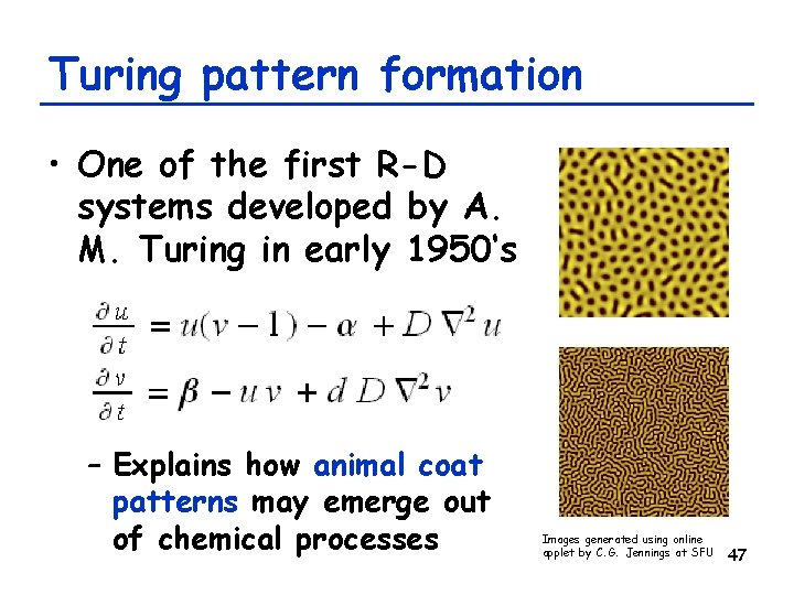
Turing pattern formation • One of the first R-D systems developed by A. M. Turing in early 1950‘s – Explains how animal coat patterns may emerge out of chemical processes Images generated using online applet by C. G. Jennings at SFU 47

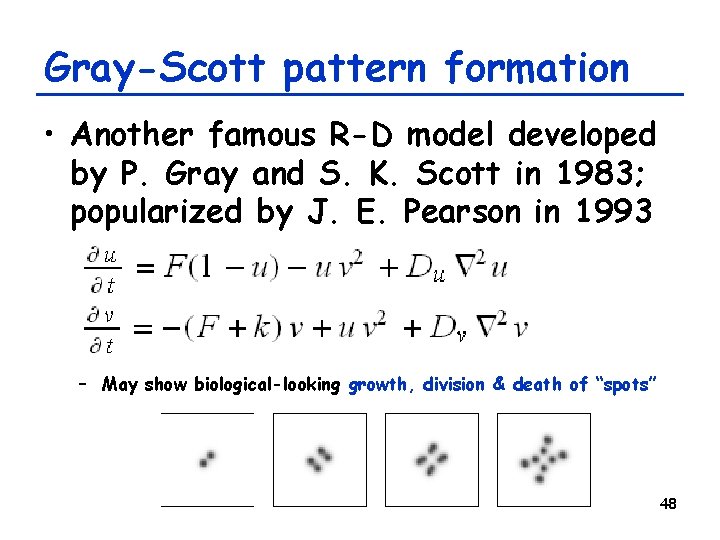
Gray-Scott pattern formation • Another famous R-D model developed by P. Gray and S. K. Scott in 1983; popularized by J. E. Pearson in 1993 – May show biological-looking growth, division & death of “spots” 48

Exercise • Study the structure of the 2 -D u-v phase spaces of BZ reaction / Turing / Gray-Scott models with no spatial distribution assumed • Obtain their equilibrium points and evaluate their stability 49

Diffusion-induced instability • Some systems have homogeneous equilibrium states which are stable if no diffusion is assumed, but which are unstable when diffusion is allowed • Mechanism that accounts for spontaneous emergence of Turing patterns 50

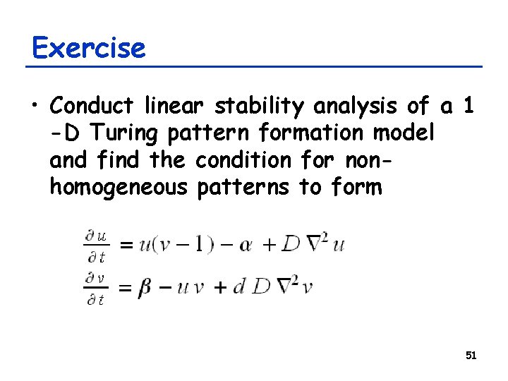
Exercise • Conduct linear stability analysis of a 1 -D Turing pattern formation model and find the condition for nonhomogeneous patterns to form 51

Summary • Spatio-temporal dynamics of complex systems may be modeled using PDEs – Typical modeling frameworks include reaction-diffusion systems • Conditions for pattern formation may be studied by conducting linear stability analysis of homogeneous equilibrium states 52