NECSI Summer School 2008 Week 3 Methods for

NECSI Summer School 2008 Week 3: Methods for the Study of Complex Systems Stochastic Systems Hiroki Sayama sayama@binghamton. edu

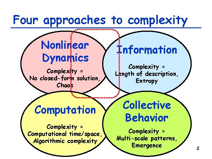
Four approaches to complexity Nonlinear Dynamics Complexity = No closed-form solution, Chaos Computation Complexity = Computational time/space, Algorithmic complexity Information Complexity = Length of description, Entropy Collective Behavior Complexity = Multi-scale patterns, Emergence 2

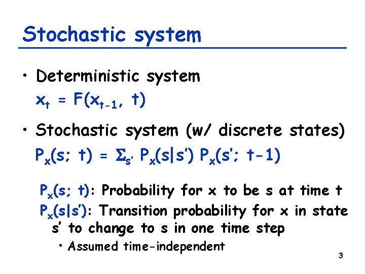
Stochastic system • Deterministic system xt = F(xt-1, t) • Stochastic system (w/ discrete states) Px(s; t) = Ss’ Px(s|s’) Px(s’; t-1) Px(s; t): Probability for x to be s at time t Px(s|s’): Transition probability for x in state s’ to change to s in one time step • Assumed time-independent 3

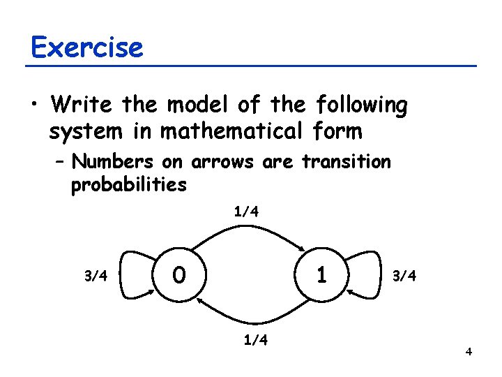
Exercise • Write the model of the following system in mathematical form – Numbers on arrows are transition probabilities 1/4 3/4 0 1 1/4 3/4 4

Random Walk 5

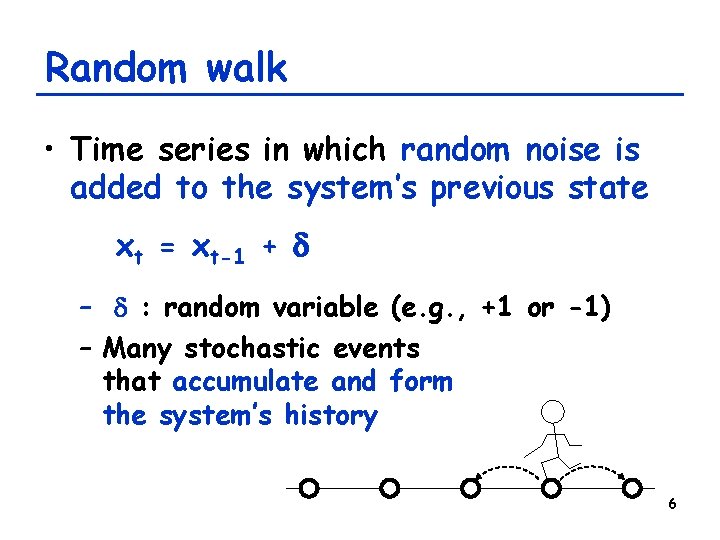
Random walk • Time series in which random noise is added to the system’s previous state xt = xt-1 + d – d : random variable (e. g. , +1 or -1) – Many stochastic events that accumulate and form the system’s history 6

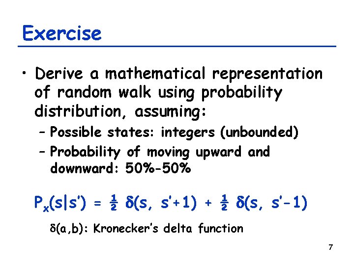
Exercise • Derive a mathematical representation of random walk using probability distribution, assuming: – Possible states: integers (unbounded) – Probability of moving upward and downward: 50%-50% Px(s|s’) = ½ d(s, s’+1) + ½ d(s, s’-1) d(a, b): Kronecker’s delta function 7

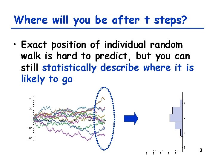
Where will you be after t steps? • Exact position of individual random walk is hard to predict, but you can still statistically describe where it is likely to go 8

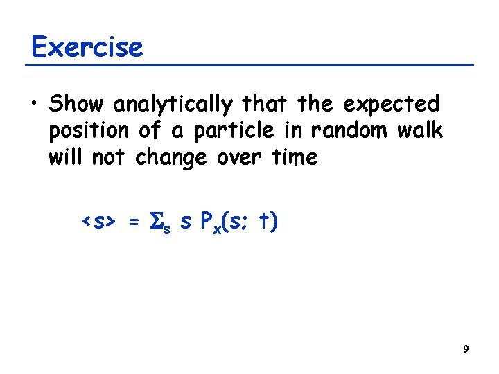
Exercise • Show analytically that the expected position of a particle in random walk will not change over time <s> = Ss s Px(s; t) 9

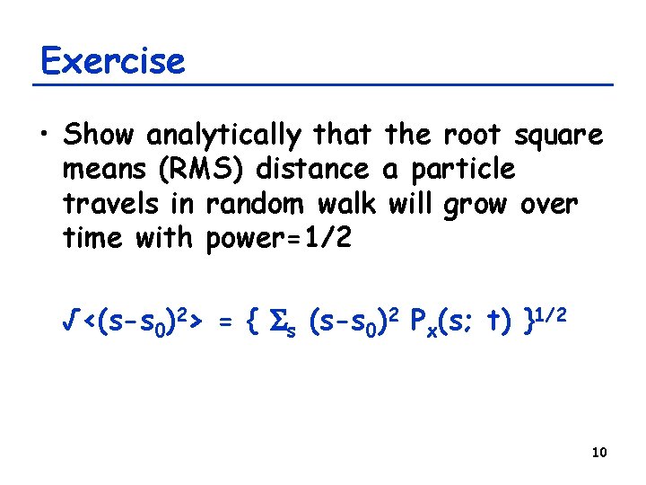
Exercise • Show analytically that the root square means (RMS) distance a particle travels in random walk will grow over time with power=1/2 √<(s-s 0)2> = { Ss (s-s 0)2 Px(s; t) }1/2 10

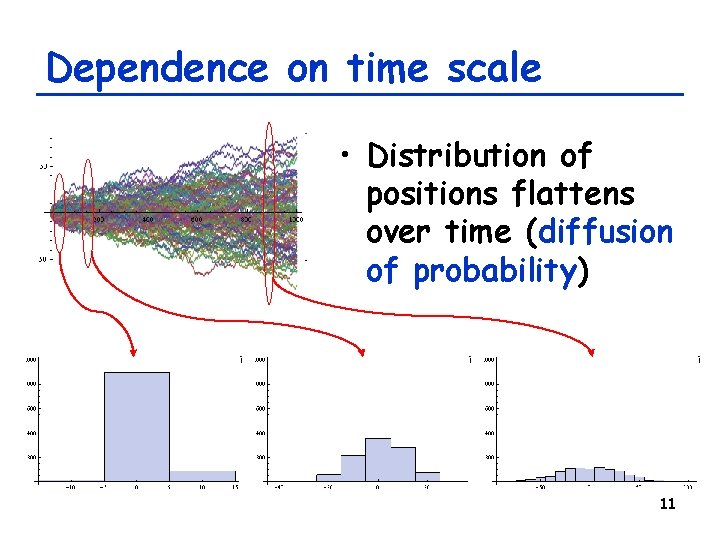
Dependence on time scale • Distribution of positions flattens over time (diffusion of probability) 11

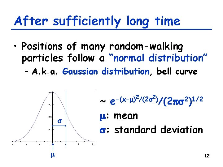
After sufficiently long time • Positions of many random-walking particles follow a “normal distribution” – A. k. a. Gaussian distribution, bell curve 2 2 -(x-m) /(2 s )/(2 ps 2)1/2 e s m ~ m: mean s: standard deviation 12

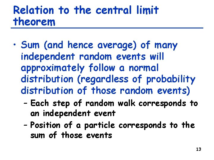
Relation to the central limit theorem • Sum (and hence average) of many independent random events will approximately follow a normal distribution (regardless of probability distribution of those random events) – Each step of random walk corresponds to an independent event – Position of a particle corresponds to the sum of those events 13

Self-Similar Properties of Individual Random Walk 14

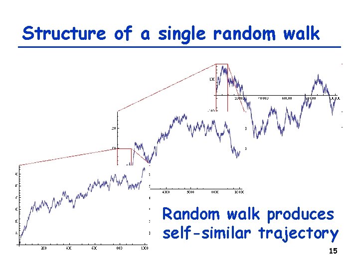
Structure of a single random walk Random walk produces self-similar trajectory 15

Fractal time series • Random walk is a very simple example of “fractal” time series – Time series whose portion has statistical properties similar to those of the whole series itself – Shows stochastic self-similarity – The word “fractal” came from the fact that these structures have fractional (non-integral) dimensions 16

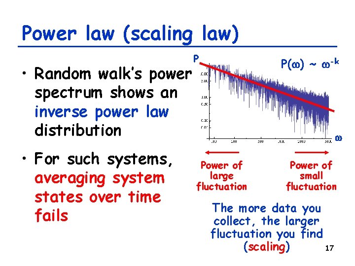
Power law (scaling law) • Random walk’s power spectrum shows an inverse power law distribution • For such systems, averaging system states over time fails P P(w) ~ w-k w Power of large fluctuation Power of small fluctuation The more data you collect, the larger fluctuation you find (scaling) 17

Exercise: Failure of averaging • Produce time series data using a random walk model • Average the system state for the first t steps • Plot this average as a function of t • Does the average become more accurate as you increase t? 18

Dynamics of fractal time series • They are always fluctuating, but not completely random • There are gentle correlations between past, present, and future (regularity) • The similar dynamics appear over a wide range of time scales, without any characteristic frequency 19

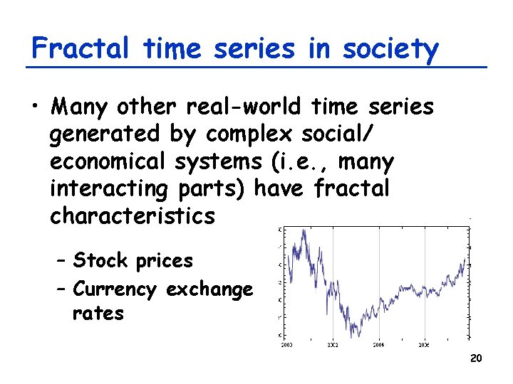
Fractal time series in society • Many other real-world time series generated by complex social/ economical systems (i. e. , many interacting parts) have fractal characteristics – Stock prices – Currency exchange rates 20

Fractal time series in biology • Many biological/physiological time series data are found to be fractal – Heartbeat rates, breathing intervals, human gaits, body temperature, etc. • They are usually fractal if a subject is normal and healthy • If they look very regular, the subject is probably not healthy • For details see, e. g. , http: //www. physionet. org/tutorials/fmnc/ 21

Transition Probability Matrix and Asymptotic Probability Distribution 22

Time evolution of probabilities • If we consider probability distribution Px(si; t) as a meta-state of the system, its time evolution is linear Px(si; t) = Sj Px(si|sj) Px(sj; t-1) pt = A pt-1 – pt: Probability vector – A: Transition probability matrix • If original state space is finite and discrete 23

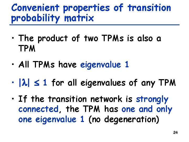
Convenient properties of transition probability matrix • The product of two TPMs is also a TPM • All TPMs have eigenvalue 1 • |l| 1 for all eigenvalues of any TPM • If the transition network is strongly connected, the TPM has one and only one eigenvalue 1 (no degeneration) 24

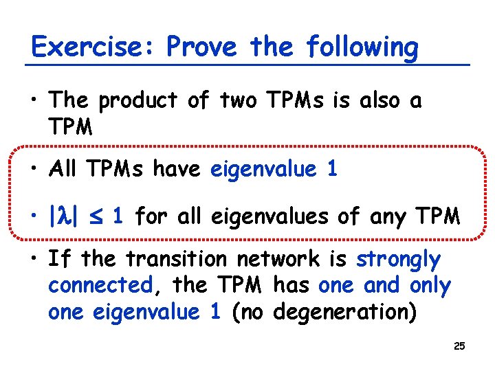
Exercise: Prove the following • The product of two TPMs is also a TPM • All TPMs have eigenvalue 1 • |l| 1 for all eigenvalues of any TPM • If the transition network is strongly connected, the TPM has one and only one eigenvalue 1 (no degeneration) 25

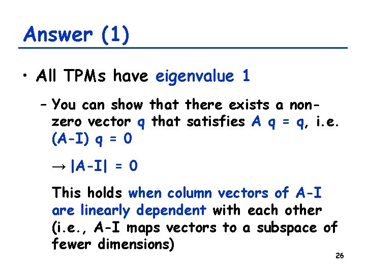
Answer (1) • All TPMs have eigenvalue 1 – You can show that there exists a nonzero vector q that satisfies A q = q, i. e. (A-I) q = 0 → |A-I| = 0 This holds when column vectors of A-I are linearly dependent with each other (i. e. , A-I maps vectors to a subspace of fewer dimensions) 26

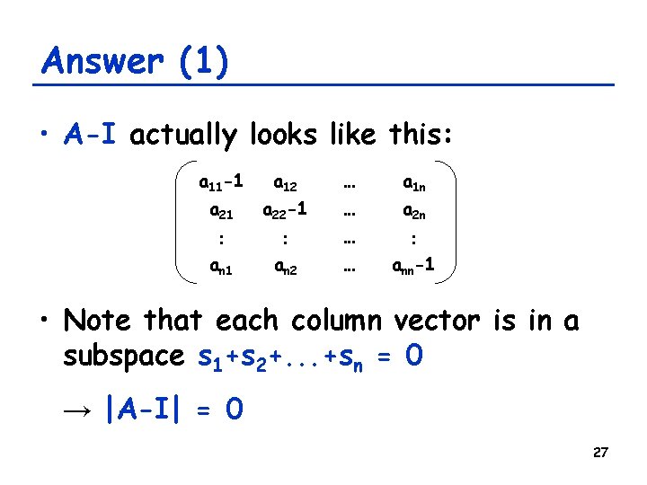
Answer (1) • A-I actually looks like this: a 11 -1 a 12 … a 1 n a 21 a 22 -1 … a 2 n ： an 1 ： an 2 … ： ann-1 … • Note that each column vector is in a subspace s 1+s 2+. . . +sn = 0 → |A-I| = 0 27

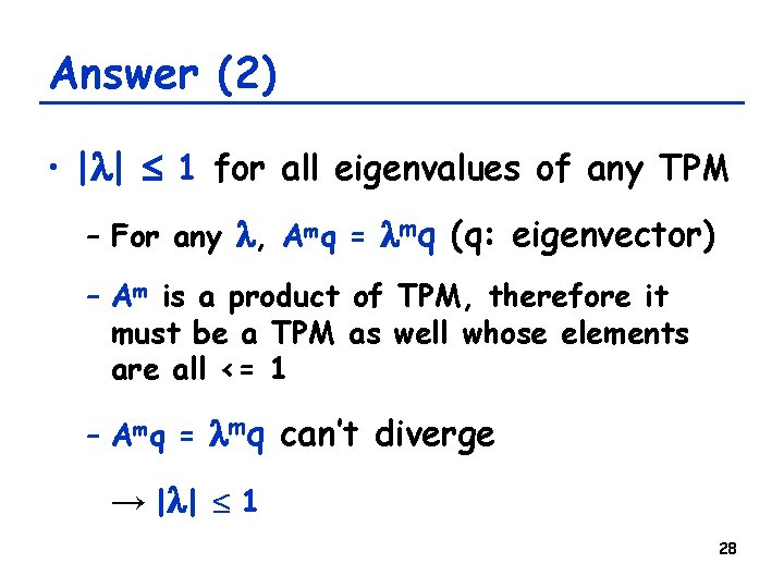
Answer (2) • |l| 1 for all eigenvalues of any TPM – For any l, Amq = lmq (q: eigenvector) – Am is a product of TPM, therefore it must be a TPM as well whose elements are all <= 1 – Amq = lmq can’t diverge → |l | 1 28

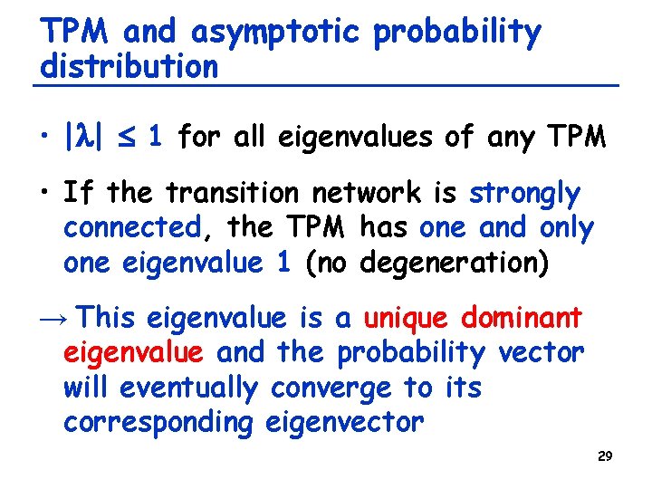
TPM and asymptotic probability distribution • |l| 1 for all eigenvalues of any TPM • If the transition network is strongly connected, the TPM has one and only one eigenvalue 1 (no degeneration) → This eigenvalue is a unique dominant eigenvalue and the probability vector will eventually converge to its corresponding eigenvector 29

An Application: Google’s “Page. Rank” 30

’s “Page. Rank” Page. Rank Explained (from http: //www. google. com/technology/) “Page. Rank relies on the uniquely democratic nature of the web by using its vast link structure as an indicator of an individual page's value. In essence, Google interprets a link from page A to page B as a vote, by page A, for page B. But, Google looks at more than the sheer volume of votes, or links a page receives; it also analyzes the page that casts the vote. Votes cast by pages that are themselves "important" weigh more heavily and help to make other 31 pages “important. ” ”

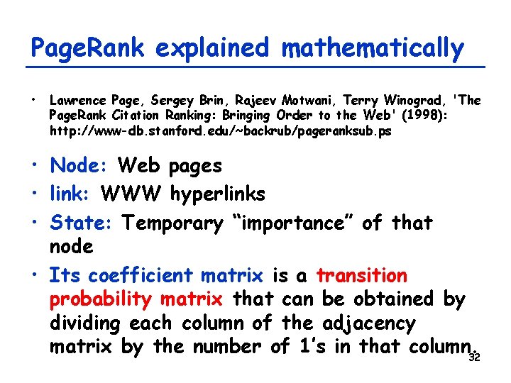
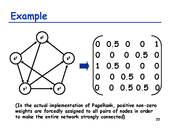
Page. Rank explained mathematically • Lawrence Page, Sergey Brin, Rajeev Motwani, Terry Winograd, 'The Page. Rank Citation Ranking: Bringing Order to the Web' (1998): http: //www-db. stanford. edu/~backrub/pageranksub. ps • Node: Web pages • link: WWW hyperlinks • State: Temporary “importance” of that node • Its coefficient matrix is a transition probability matrix that can be obtained by dividing each column of the adjacency matrix by the number of 1’s in that column. 32

Example s 1 s 2 s 5 s 3 s 4 0 0. 5 0 0 0. 5 1 0. 5 0 0 0 0. 5 1 0 0 (In the actual implementation of Page. Rank, positive non-zero weights are forcedly assigned to all pairs of nodes in order to make the entire network strongly connected) 33

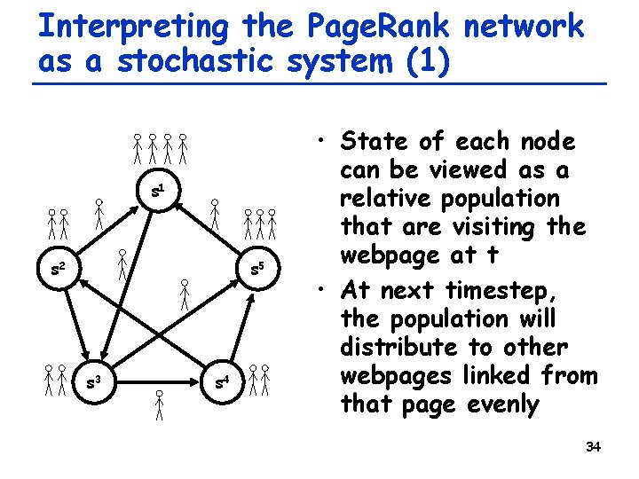
Interpreting the Page. Rank network as a stochastic system (1) s 1 s 2 s 5 s 3 s 4 • State of each node can be viewed as a relative population that are visiting the webpage at t • At next timestep, the population will distribute to other webpages linked from that page evenly 34

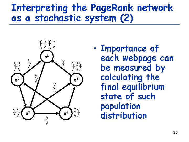
Interpreting the Page. Rank network as a stochastic system (2) s 1 s 2 s 5 s 3 s 4 • Importance of each webpage can be measured by calculating the final equilibrium state of such population distribution 35

Therefore. . . • Just one dominant eigenvector of the TPM of a strongly connected network always exists, with l = 1 • This shows the equilibrium distribution of the population over WWW • So, just solve x = Ax and you will get the Page. Rank for all the web pages on the World Wide Web!! 36

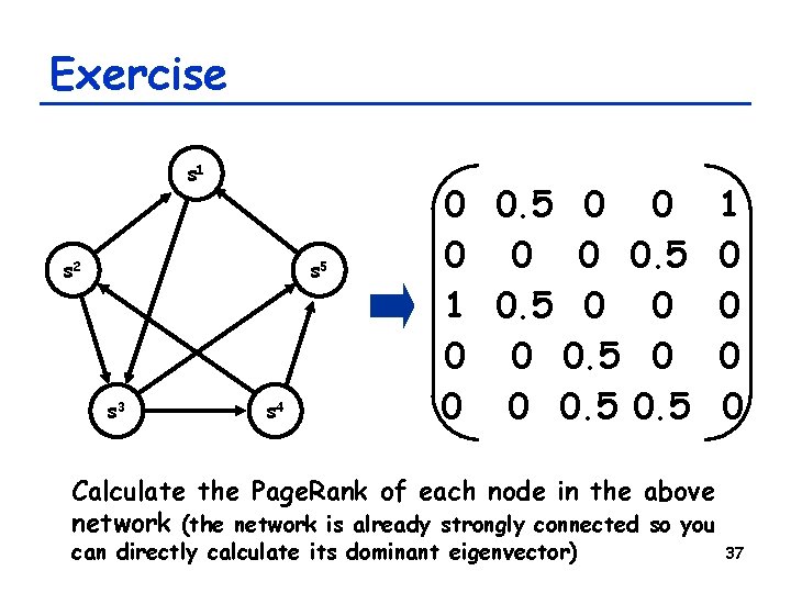
Exercise s 1 s 2 s 5 s 3 s 4 0 0. 5 0 0 0. 5 1 0. 5 0 0 0 0. 5 1 0 0 Calculate the Page. Rank of each node in the above network (the network is already strongly connected so you can directly calculate its dominant eigenvector) 37

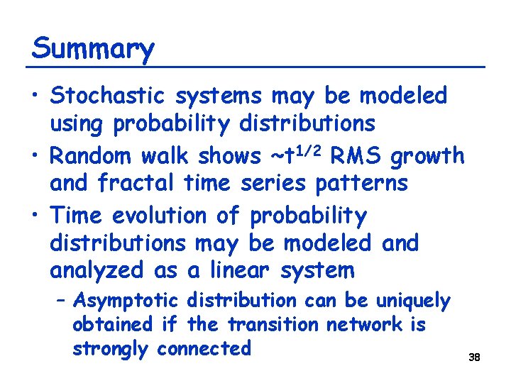
Summary • Stochastic systems may be modeled using probability distributions • Random walk shows ~t 1/2 RMS growth and fractal time series patterns • Time evolution of probability distributions may be modeled analyzed as a linear system – Asymptotic distribution can be uniquely obtained if the transition network is strongly connected 38

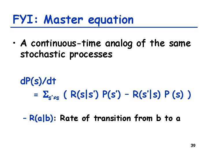
FYI: Master equation • A continuous-time analog of the same stochastic processes d. P(s)/dt = Ss’≠s ( R(s|s’) P(s’) – R(s’|s) P (s) ) – R(a|b): Rate of transition from b to a 39