NECSI Summer School 2008 Week 2 Complex Systems

NECSI Summer School 2008 Week 2: Complex Systems Modeling and Networks Non-Spatial Models Hiroki Sayama sayama@binghamton. edu

Dynamical systems approach • A system whose state is uniquely specified by a finite set of variables and whose behavior is uniquely determined by predetermined rules – – Simple population growth Simple pendulum swinging Motion of celestial bodies Behavior of two “rational” agents in a negotiation game 2

Mathematical formulations of dynamical systems • Discrete-time model: (difference/recurrence equations; iterative maps) xt = F(xt-1, t) • Continuous-time model: (differential equations) dx/dt = F(x, t) xt: State variable of the system at time t • May take “scalar” or “vector” value F: Some function that determines the rule that the system’s behavior will obey 3

Discrete-Time Models 4

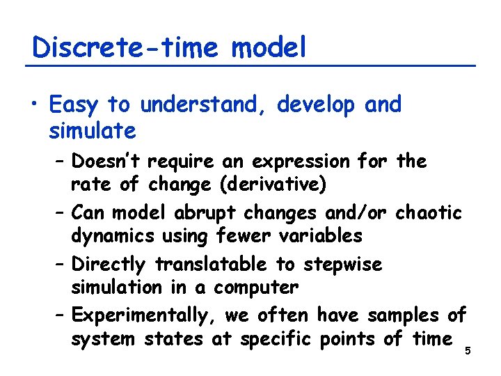
Discrete-time model • Easy to understand, develop and simulate – Doesn’t require an expression for the rate of change (derivative) – Can model abrupt changes and/or chaotic dynamics using fewer variables – Directly translatable to stepwise simulation in a computer – Experimentally, we often have samples of system states at specific points of time 5

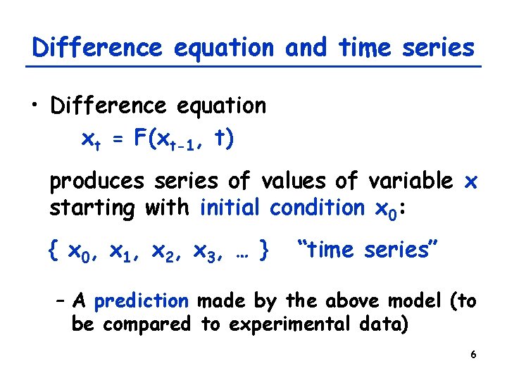
Difference equation and time series • Difference equation xt = F(xt-1, t) produces series of values of variable x starting with initial condition x 0: { x 0, x 1, x 2, x 3, … } “time series” – A prediction made by the above model (to be compared to experimental data) 6

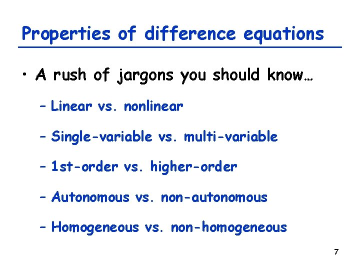
Properties of difference equations • A rush of jargons you should know… – Linear vs. nonlinear – Single-variable vs. multi-variable – 1 st-order vs. higher-order – Autonomous vs. non-autonomous – Homogeneous vs. non-homogeneous 7

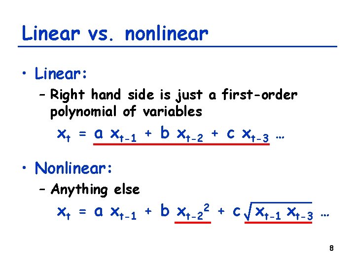
Linear vs. nonlinear • Linear: – Right hand side is just a first-order polynomial of variables xt = a xt-1 + b xt-2 + c xt-3 … • Nonlinear: – Anything else xt = a xt-1 + b xt-22 + c xt-1 xt-3 … 8

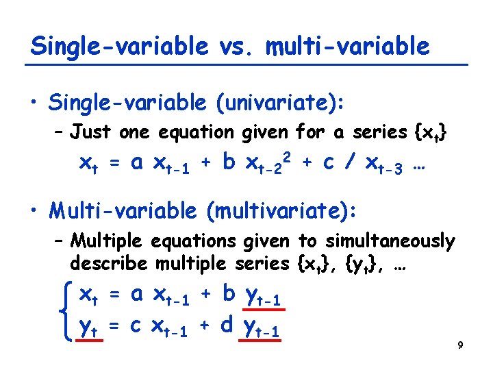
Single-variable vs. multi-variable • Single-variable (univariate): – Just one equation given for a series {xt} xt = a xt-1 + b xt-22 + c / xt-3 … • Multi-variable (multivariate): – Multiple equations given to simultaneously describe multiple series {xt}, {yt}, … xt = a xt-1 + b yt-1 yt = c xt-1 + d yt-1 9

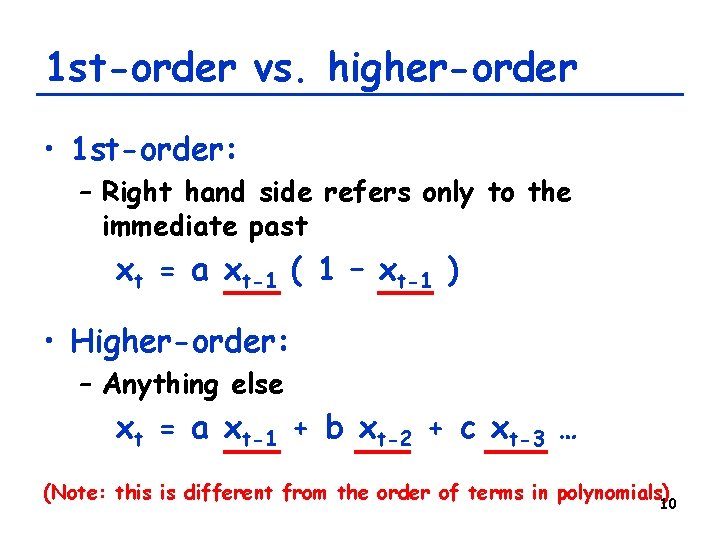
1 st-order vs. higher-order • 1 st-order: – Right hand side refers only to the immediate past xt = a xt-1 ( 1 – xt-1 ) • Higher-order: – Anything else xt = a xt-1 + b xt-2 + c xt-3 … (Note: this is different from the order of terms in polynomials) 10

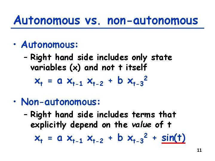
Autonomous vs. non-autonomous • Autonomous: – Right hand side includes only state variables (x) and not t itself xt = a xt-1 xt-2 + b xt-32 • Non-autonomous: – Right hand side includes terms that explicitly depend on the value of t xt = a xt-1 xt-2 + b xt-32 + sin(t) 11

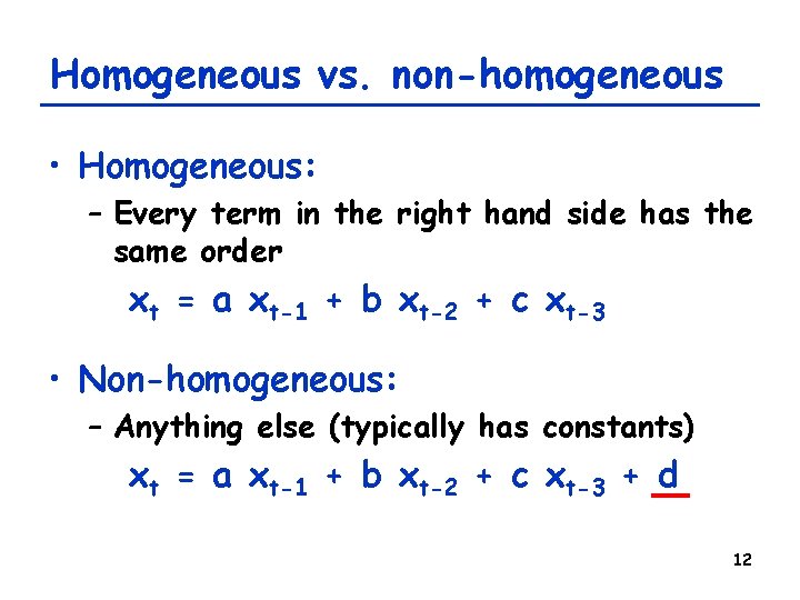
Homogeneous vs. non-homogeneous • Homogeneous: – Every term in the right hand side has the same order xt = a xt-1 + b xt-2 + c xt-3 • Non-homogeneous: – Anything else (typically has constants) xt = a xt-1 + b xt-2 + c xt-3 + d 12

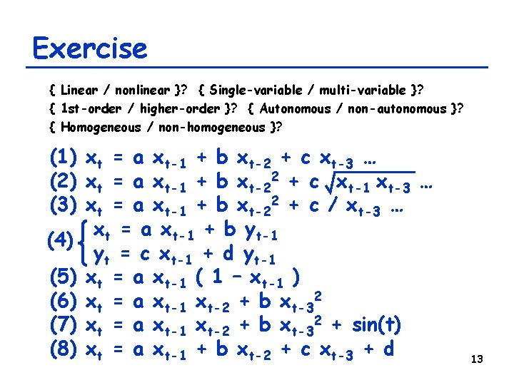
Exercise { Linear / nonlinear }? { Single-variable / multi-variable }? { 1 st-order / higher-order }? { Autonomous / non-autonomous }? { Homogeneous / non-homogeneous }? (1) xt = a xt-1 + b xt-2 + c xt-3 … (2) xt = a xt-1 + b xt-22 + c xt-1 xt-3 … (3) xt = a xt-1 + b xt-22 + c / xt-3 … xt = a xt-1 + b yt-1 (4) yt = c xt-1 + d yt-1 (5) xt = a xt-1 ( 1 – xt-1 ) (6) xt = a xt-1 xt-2 + b xt-32 (7) xt = a xt-1 xt-2 + b xt-32 + sin(t) (8) xt = a xt-1 + b xt-2 + c xt-3 + d 13

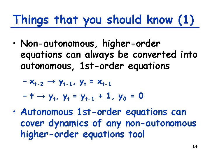
Things that you should know (1) • Non-autonomous, higher-order equations can always be converted into autonomous, 1 st-order equations – xt-2 → yt-1, yt = xt-1 – t → yt, yt = yt-1 + 1, y 0 = 0 • Autonomous 1 st-order equations can cover dynamics of any non-autonomous higher-order equations too! 14

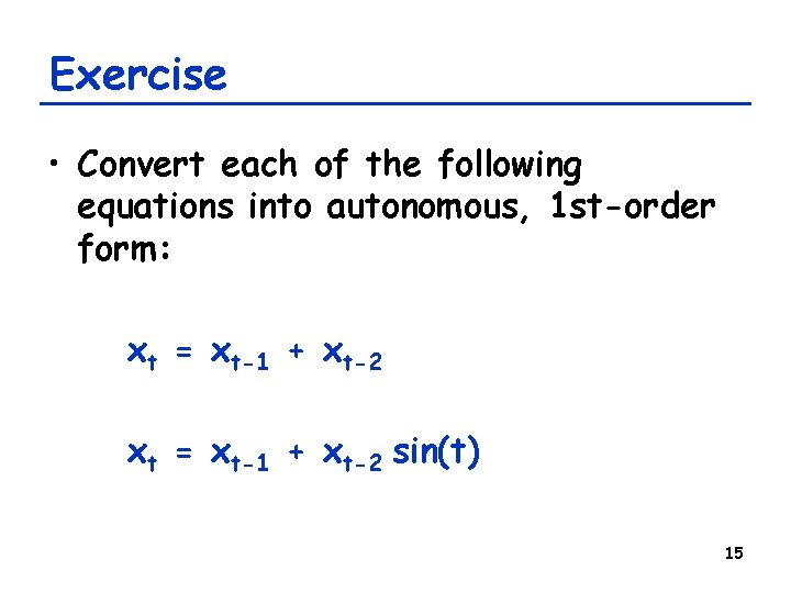
Exercise • Convert each of the following equations into autonomous, 1 st-order form: xt = xt-1 + xt-2 sin(t) 15

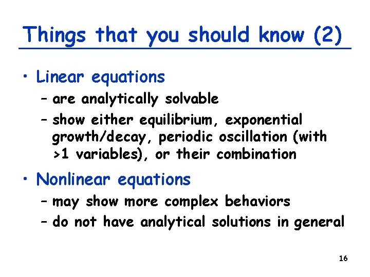
Things that you should know (2) • Linear equations – are analytically solvable – show either equilibrium, exponential growth/decay, periodic oscillation (with >1 variables), or their combination • Nonlinear equations – may show more complex behaviors – do not have analytical solutions in general 16

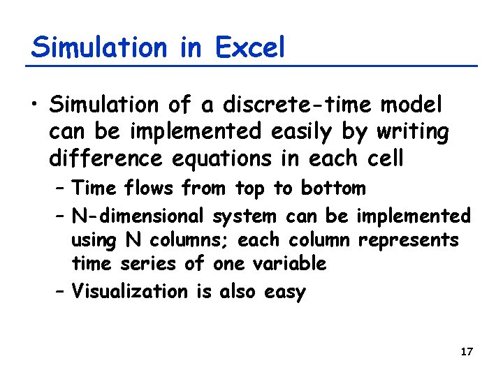
Simulation in Excel • Simulation of a discrete-time model can be implemented easily by writing difference equations in each cell – Time flows from top to bottom – N-dimensional system can be implemented using N columns; each column represents time series of one variable – Visualization is also easy 17

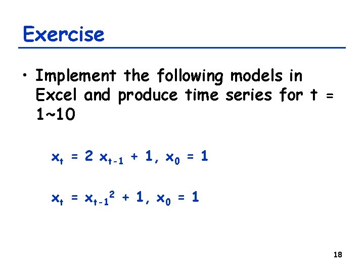
Exercise • Implement the following models in Excel and produce time series for t = 1~10 xt = 2 xt-1 + 1, x 0 = 1 xt = xt-12 + 1, x 0 = 1 18

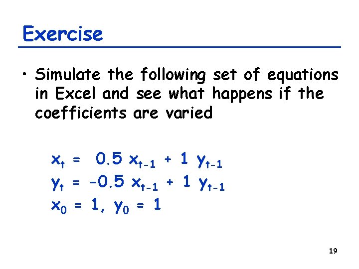
Exercise • Simulate the following set of equations in Excel and see what happens if the coefficients are varied xt = 0. 5 xt-1 + 1 yt-1 yt = -0. 5 xt-1 + 1 yt-1 x 0 = 1, y 0 = 1 19

Developing Discrete-Time Models with One Variable 20

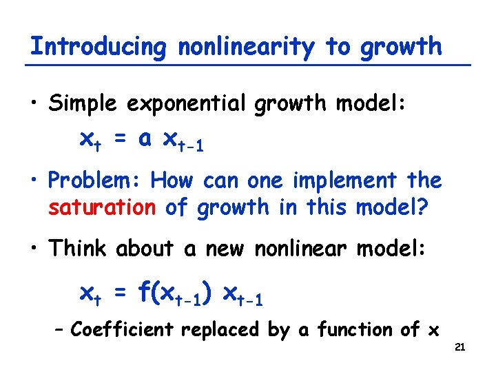
Introducing nonlinearity to growth • Simple exponential growth model: xt = a xt-1 • Problem: How can one implement the saturation of growth in this model? • Think about a new nonlinear model: xt = f(xt-1) xt-1 – Coefficient replaced by a function of x 21

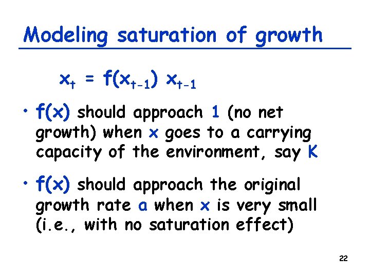
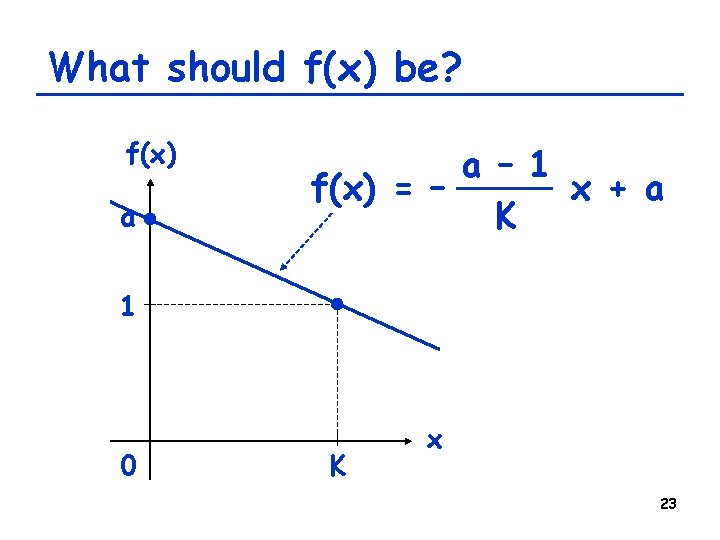
Modeling saturation of growth xt = f(xt-1) xt-1 • f(x) should approach 1 (no net growth) when x goes to a carrying capacity of the environment, say K • f(x) should approach the original growth rate a when x is very small (i. e. , with no saturation effect) 22

What should f(x) be? f(x) a a – 1 f(x) = – x + a K 1 0 K x 23

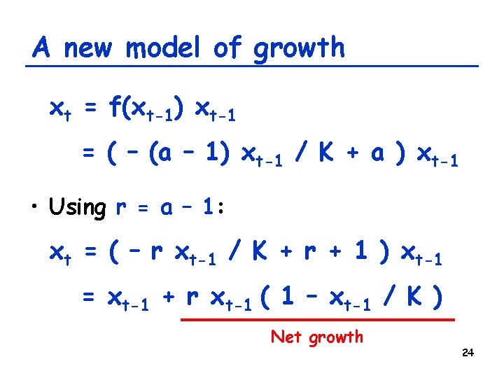
A new model of growth xt = f(xt-1) xt-1 = ( – (a – 1) xt-1 / K + a ) xt-1 • Using r = a – 1: xt = ( – r xt-1 / K + r + 1 ) xt-1 = xt-1 + r xt-1 ( 1 – xt-1 / K ) Net growth 24

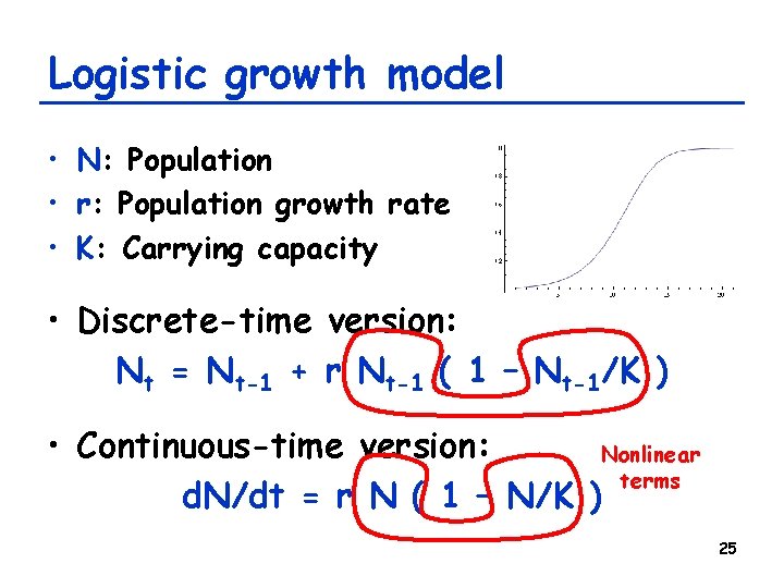
Logistic growth model • N: Population • r: Population growth rate • K: Carrying capacity • Discrete-time version: Nt = Nt-1 + r Nt-1 ( 1 – Nt-1/K ) • Continuous-time version: Nonlinear terms d. N/dt = r N ( 1 – N/K ) 25

Exercise • Simulate the behavior of the logistic growth model using Excel with 0 < r < 3, K = 1, N 0 = 0. 01 • Consider if the same behavior can be achieved by a linear model – If not, how is it different? 26

Logistic Map and Chaos 27

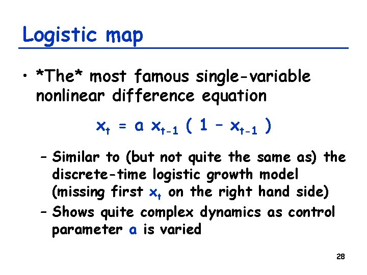
Logistic map • *The* most famous single-variable nonlinear difference equation xt = a xt-1 ( 1 – xt-1 ) – Similar to (but not quite the same as) the discrete-time logistic growth model (missing first xt on the right hand side) – Shows quite complex dynamics as control parameter a is varied 28

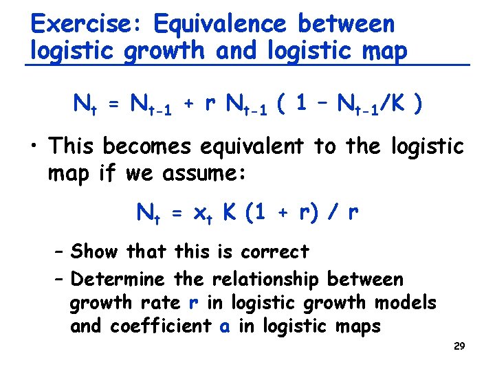
Exercise: Equivalence between logistic growth and logistic map Nt = Nt-1 + r Nt-1 ( 1 – Nt-1/K ) • This becomes equivalent to the logistic map if we assume: Nt = xt K (1 + r) / r – Show that this is correct – Determine the relationship between growth rate r in logistic growth models and coefficient a in logistic maps 29

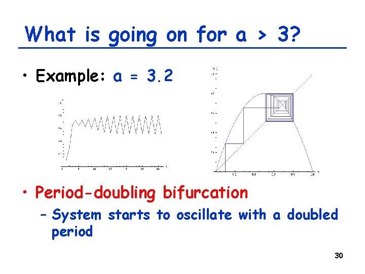
What is going on for a > 3? • Example: a = 3. 2 • Period-doubling bifurcation – System starts to oscillate with a doubled period 30

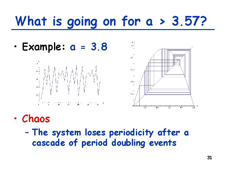
What is going on for a > 3. 57? • Example: a = 3. 8 • Chaos – The system loses periodicity after a cascade of period doubling events 31

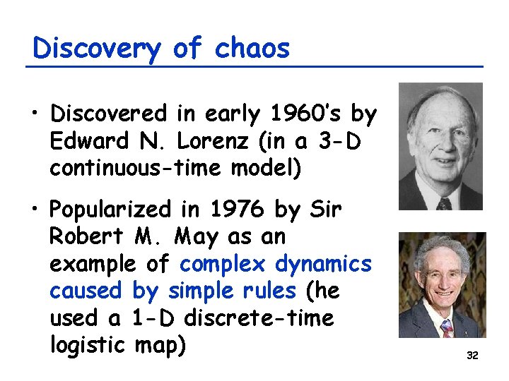
Discovery of chaos • Discovered in early 1960’s by Edward N. Lorenz (in a 3 -D continuous-time model) • Popularized in 1976 by Sir Robert M. May as an example of complex dynamics caused by simple rules (he used a 1 -D discrete-time logistic map) 32

Chaos in dynamical systems • A long-term behavior of a dynamical system that never falls in any static or periodic trajectories • Looks like a random fluctuation, but still occurs in completely deterministic simple systems • Exhibits sensitivity to initial conditions • Can be found everywhere 33

Take-home lessons • Complexity does NOT require complex underlying rule structure – Simple deterministic systems may show complex behavior if they are nonlinear • Nonlinear systems often entail chaos in their dynamics – This is why analytical solutions are not available for nonlinear systems 34

Developing Discrete-Time Models with Multiple Variables 35

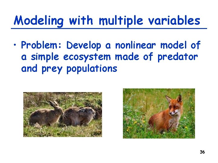
Modeling with multiple variables • Problem: Develop a nonlinear model of a simple ecosystem made of predator and prey populations 36

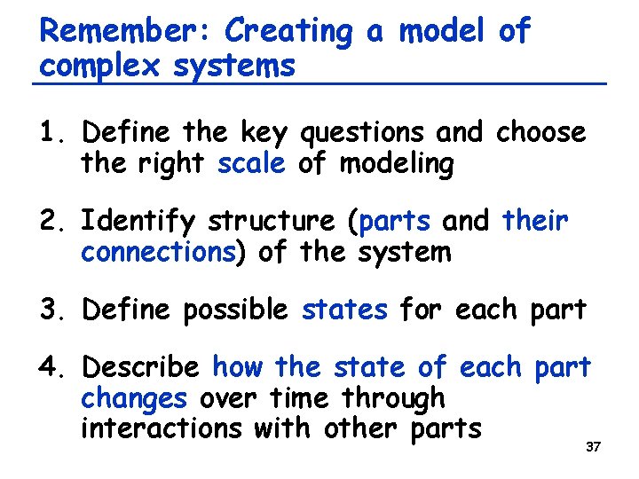
Remember: Creating a model of complex systems 1. Define the key questions and choose the right scale of modeling 2. Identify structure (parts and their connections) of the system 3. Define possible states for each part 4. Describe how the state of each part changes over time through interactions with other parts 37

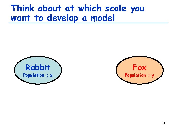
Think about at which scale you want to develop a model Rabbit Population : x Fox Population : y 38

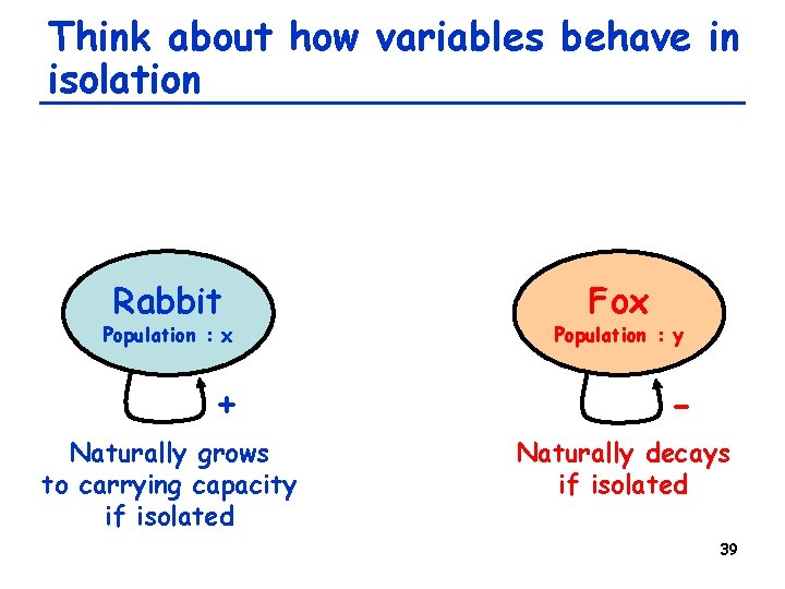
Think about how variables behave in isolation Rabbit Population : x + Naturally grows to carrying capacity if isolated Fox Population : y Naturally decays if isolated 39

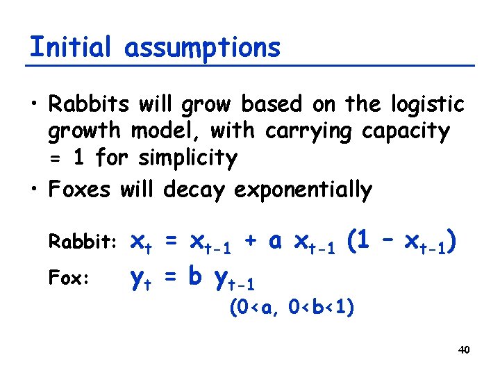
Initial assumptions • Rabbits will grow based on the logistic growth model, with carrying capacity = 1 for simplicity • Foxes will decay exponentially Rabbit: Fox: xt = xt-1 + a xt-1 (1 – xt-1) yt = b yt-1 (0<a, 0<b<1) 40

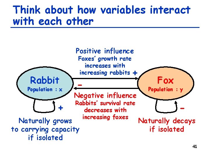
Think about how variables interact with each other Positive influence Rabbit Population : x + Foxes’ growth rate increases with increasing rabbits - + Negative influence Rabbits’ survival rate decreases with increasing foxes Naturally grows to carrying capacity if isolated Fox Population : y Naturally decays if isolated 41

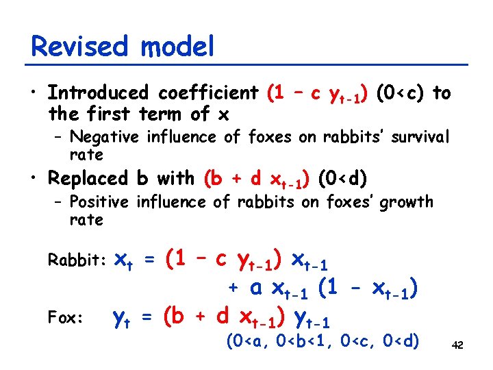
Revised model • Introduced coefficient (1 – c yt-1) (0<c) to the first term of x – Negative influence of foxes on rabbits’ survival rate • Replaced b with (b + d xt-1) (0<d) – Positive influence of rabbits on foxes’ growth rate Rabbit: Fox: xt = (1 – c yt-1) xt-1 + a xt-1 (1 - xt-1) yt = (b + d xt-1) yt-1 (0<a, 0<b<1, 0<c, 0<d) 42

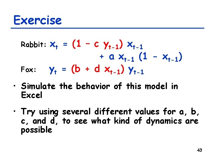
Exercise Rabbit: Fox: xt = (1 – c yt-1) xt-1 + a xt-1 (1 - xt-1) yt = (b + d xt-1) yt-1 • Simulate the behavior of this model in Excel • Try using several different values for a, b, c, and d, to see what kind of dynamics are possible 43

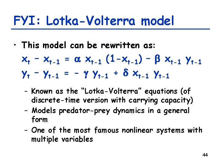
FYI: Lotka-Volterra model • This model can be rewritten as: xt – xt-1 = a xt-1 (1 -xt-1) – b xt-1 yt – yt-1 = - g yt-1 + d xt-1 yt-1 – Known as the “Lotka-Volterra” equations (of discrete-time version with carrying capacity) – Models predator-prey dynamics in a general form – One of the most famous nonlinear systems with multiple variables 44

Continuous-Time Models 45

Mathematical formulations of dynamical systems • Discrete-time model: (difference/recurrence equations; iterative maps) xt = F(xt-1, t) • Continuous-time model: (differential equations) dx/dt = F(x, t) xt: State variable of the system at time t • May take “scalar” or “vector” value F: Some function that determines the rule that the system’s behavior will obey 46

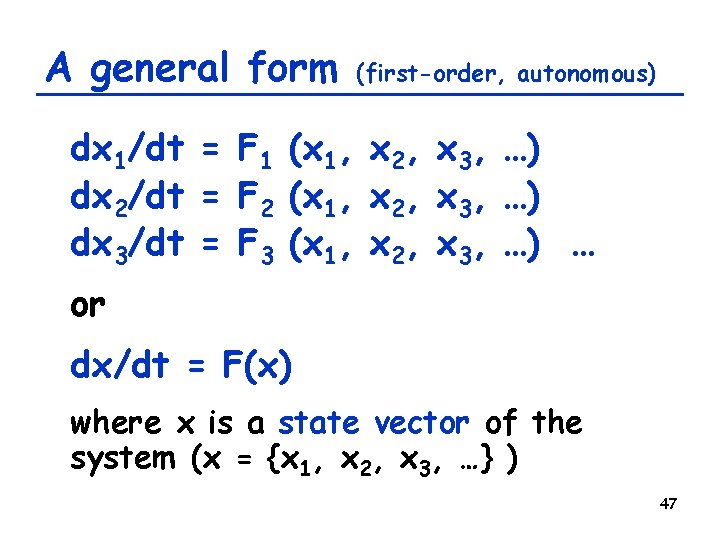
A general form (first-order, autonomous) dx 1/dt = F 1 (x 1, x 2, x 3, …) dx 2/dt = F 2 (x 1, x 2, x 3, …) dx 3/dt = F 3 (x 1, x 2, x 3, …) … or dx/dt = F(x) where x is a state vector of the system (x = {x 1, x 2, x 3, …} ) 47

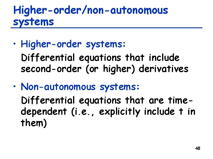
Higher-order/non-autonomous systems • Higher-order systems: Differential equations that include second-order (or higher) derivatives • Non-autonomous systems: Differential equations that are timedependent (i. e. , explicitly include t in them) 48

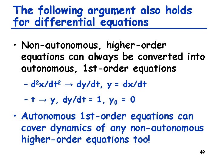
The following argument also holds for differential equations • Non-autonomous, higher-order equations can always be converted into autonomous, 1 st-order equations – d 2 x/dt 2 → dy/dt, y = dx/dt – t → y, dy/dt = 1, y 0 = 0 • Autonomous 1 st-order equations can cover dynamics of any non-autonomous higher-order equations too! 49

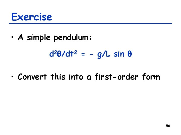
Exercise • A simple pendulum: d 2 q/dt 2 = - g/L sin q • Convert this into a first-order form 50

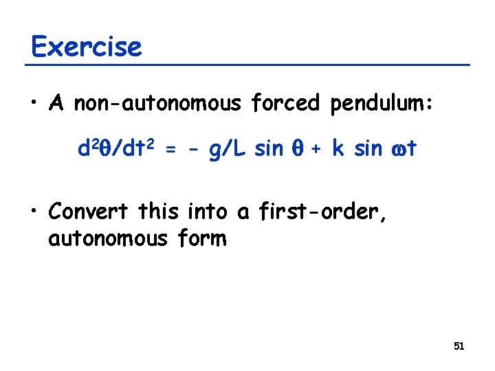
Exercise • A non-autonomous forced pendulum: d 2 q/dt 2 = - g/L sin q + k sin wt • Convert this into a first-order, autonomous form 51

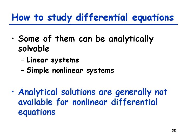
How to study differential equations • Some of them can be analytically solvable – Linear systems – Simple nonlinear systems • Analytical solutions are generally not available for nonlinear differential equations 52

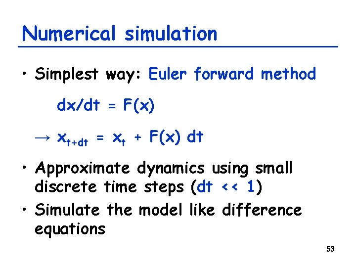
Numerical simulation • Simplest way: Euler forward method dx/dt = F(x) → xt+dt = xt + F(x) dt • Approximate dynamics using small discrete time steps (dt << 1) • Simulate the model like difference equations 53

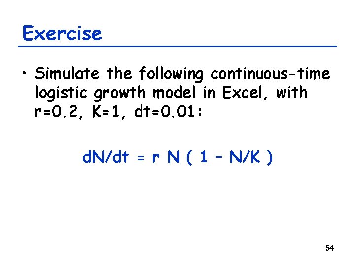
Exercise • Simulate the following continuous-time logistic growth model in Excel, with r=0. 2, K=1, dt=0. 01: d. N/dt = r N ( 1 – N/K ) 54

Modeling Exercises 55

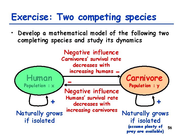
Exercise: Two competing species • Develop a mathematical model of the following two completing species and study its dynamics Negative influence Human Carnivores’ survival rate decreases with increasing humans Population : x + Naturally grows if isolated - - Negative influence Humans’ survival rate decreases with increasing carnivores Carnivore Population : y + Naturally grows if isolated (assume plenty of 56 prey are available)

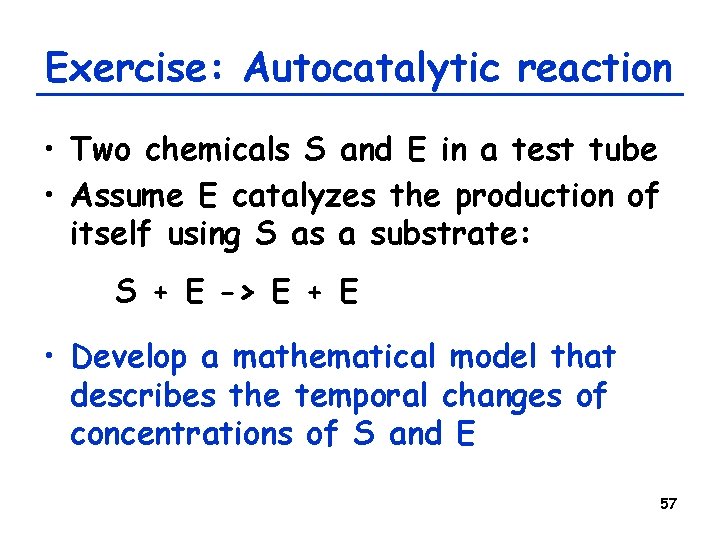
Exercise: Autocatalytic reaction • Two chemicals S and E in a test tube • Assume E catalyzes the production of itself using S as a substrate: S + E -> E + E • Develop a mathematical model that describes the temporal changes of concentrations of S and E 57

Exercise: Rise and fall of songs • When a new pop song is released, it sounds attractive to people and its popularity increases (maybe depending on the quality of the song too) • After people get used to the song, it begins to bore them and eventually gets taken over by other new songs • Develop a mathematical model that captures such rise and fall in a typical pop song’s life 58

Exercise: Blood type distribution • Human blood types are determined by the combination of three different alleles, A, B and O (Possible genotypes: AA, AB, AO, BB, BO, OO) • Each parent gives one of his/her two alleles to a child • Model and study how the blood type distribution changes over many generations (with the assumption that there is no selection acting on them) 59