Introduction to Genomics and the Tree of Life

Introduction to Genomics and the Tree of Life (part 2) Monday, October 25, 2010 Genomics 260. 605. 01 J. Pevsner pevsner@kennedykrieger. org

Outline of this course Tree of life Viruses Bacteria and archaea (Egbert Hoiczyk) Eukaryotes The eukaryotic chromosome Fungi; yeast functional genomics (Jef Boeke) Protozoans (David Sullivan) Nematodes (Alan Scott) Rodents: mouse and rat Primates The human genome (Dave Valle) Human disease

Five approaches to genomics As we survey the tree of life, consider these perspectives: Approach I: cataloguing genomic information Genome size; number of chromosomes; GC content; isochores; number of genes; repetitive DNA; unique features of each genome Approach II: cataloguing comparative genomic information Orthologs and paralogs; COGs; lateral gene transfer Approach III: function; biological principles; evolution How genome size is regulated; polyploidization; birth and death of genes; neutral theory of evolution; positive and negative selection; speciation Approach IV: Human disease relevance Approach V: Bioinformatics aspects Algorithms, databases, websites

Pace (2001) described a tree of life based on small subunit r. RNA sequences. This tree shows the main three branches described by Woese and colleagues. Fig. 13. 1 Page 521

Outline of what we covered in Friday’s lecture Introduction: 5 perspectives, history of life: time lines Genome-sequencing projects: chronology Genome analysis: criteria, resequencing, metagenomics DNA sequencing technologies: Sanger, 454, Solexa Process of genome sequencing: centers, repositories Genome annotation: features, prokaryotes, eukaryotes

Learning objectives for today 1. You should be able to describe these aspects of genome analysis: criteria, resequencing, metagenomics 2. You should understand how one next-generation DNA sequencing technology is performed 3. You should be able to describe the process of genome sequencing: centers, repositories 4. You should be able to describe basic features of genome annotation for prokaryotes and eukaryotes

Completed genome projects (current 10/10) Eukaryotes: 37 complete; 350 assembly, 505 in progress Viruses: 3, 110 complete Bacteria: 1, 163 complete Archaea: 91 complete Organellar: 2, 487 complete Metagenomics projects: 306 Page 527, 537

Learning objectives from Friday’s lecture (first half of Chapter 13) • Describe five perspectives on genomics (cataloguing information, comparative genomics, biological principles, disease relevance, bioinformatics aspects) • Provide a rough chronology of the history of life on earth (this will become easier as the course progresses) • Provide a rough chronology of genome-sequencing projects • Use key NCBI resources to find information about genomes

Outline of today’s lecture Introduction: 5 perspectives, history of life Genome-sequencing projects: chronology Genome analysis: criteria, resequencing, metagenomics DNA sequencing technologies: Sanger, 454, Solexa Process of genome sequencing: centers, repositories Genome annotation: features, prokaryotes, eukaryotes

Learning objectives for today’s lecture (Chapter 13, second half) • Explain the major applications of next-generation sequencing including resequencing and metagenomics • Describe how next-generation sequencing technologies work (we will examine NGS data later) • Define the major repositories of DNA sequence data and search one (the Trace Archive) for particular sequences such as human beta globin

Overview of genome analysis • Selection of genomes for sequencing • Sequence one individual genome, or several? • How big are genomes? • Genome sequencing centers • Sequencing genomes: strategies • When has a genome been fully sequenced? • Repository for genome sequence data • Genome annotation Page 537

Applications of Genome Sequencing Purpose Template Example De novo sequencing Genome sequencing Sequencing genomes Ancient DNA Extinct Neanderthal genome Metagenomics Human gut Resequencing Whole genomes Genomic regions Somatic mutations Transcriptome Full-length transcripts Serial Analysis of Gene Expression (SAGE) Epigenetics >1000 influenza Individual humans Assessment of genomic rearrangements or diseaseassociated regions Sequencing mutations in cancer Defining regulated messenger RNA transcripts Noncoding RNAs Identifying and quantifying micro. RNAs in samples Methylation changes Measuring methylation changes in cancer Table 13. 15 p. 538

Overview of genome analysis Fig. 13. 8 p. 539

Criteria for selecting genomes for sequencing Criteria include: • genome size (some plants are >>>human genome) • cost • relevance to human disease (or other disease) • relevance to basic biological questions • relevance to agriculture Page 538

Criteria for selecting genomes for sequencing Criteria include: • genome size (some plants are >>>human genome) • cost • relevance to human disease (or other disease) • relevance to basic biological questions • relevance to agriculture Recent projects: Chicken Chimpanzee Cow Dog Fungi (many) Honey bee Sea urchin Rhesus macaque Page 540

Selection criteria Selection of genomes for sequencing is based on specific criteria. For an overview, see a series of white papers posted on the National Human Genome Research Institute (NHGRI) website: http: //www. genome. gov/10002154 For a description of NHGRI selection criteria, visit: http: //www. genome. gov/10001495 Page 540

Criteria for selecting genomes for sequencing Sequence one individual genome, or several? Try one… --Each genome center may study one chromosome from an organism --It is necessary to measure polymorphisms (e. g. SNPs) in large populations For viruses, thousands of isolates may be sequenced. For the human genome, cost is the impediment. Page 540

Diversity of genome sizes How big are genomes? Viral genomes: 1 kb to 350 kb (Mimivirus: 1181 kb) Bacterial genomes: 0. 5 Mb to 13 Mb Eukaryotic genomes: 8 Mb to 686 Gb (human: ~3 Gb) Page 540

Genome sizes in nucleotide base pairs plasmids viruses bacteria fungi plants algae insects mollusks bony fish The size of the human genome is ~ 3 X 109 bp; almost all of its complexity is in single-copy DNA. amphibians reptiles The human genome is thought to contain ~30, 000 -40, 000 genes. 104 105 106 107 birds mammals 108 109 1010 1011 http: //www 3. kumc. edu/jcalvet/Power. Point/bioc 801 b. ppt

Entrez Genomes at NCBI (September 2006): sizes of 197 sequenced eukaryotic genomes 4000 genome size (megabases) 3000 2000 1000 0 0 100 number Updated 9/06 200

16 eukaryotic genome projects > 1000 megabases Genus, species Subgroup Size (Mb) #chr common name Macropus eugenii Mammals 3800 8 tammar wallaby Oryctolagus cuniculus Mammals 3500 22 rabbit Cavia porcellus Mammals 3400 31 guinea pig Pan troglodytes Mammals 3100 24 chimpanzee Homo sapiens Mammals 3038 23 human Bos taurus Mammals 3000 30 cow Dasypus novemcinctus Mammals 3000 32 nine-banded armadillo Loxodonta africana Mammals 3000 28 African savanna elephant Sorex araneus Mammals 3000 Rattus norvegicus Mammals 2750 21 rat Canis familiaris Mammals 2400 39 dog Zea mays Land Plants 2365 10 corn Aplysia californica Other Animals 1800 17 California sea hare Danio rerio Fishes 1700 25 zebrafish Gallus gallus Birds 1200 40 chicken Triphysaria versicolor Land Plants 1200 European shrew plant parasite

Entrez Genomes at NCBI (September 2006): 100 smallest sequenced eukaryotic genomes 50 40 genome size 30 (megabases) 20 10 0 0 50 number 100 These 100 genomes consist of fungi (n=76), plants (n=2), and protists (n=22). Updated 9/06

Smallest eukaryotic genome projects Name Group Size (Mb) #Chr Encephalitozoon cuniculi Fungi 2. 5 11 Antonospora locustae Fungi 2. 9 Leishmania major Friedlin Protists 5. 44 Pneumocystis carinii Fungi 8 Cryptosporidium hominis Protists 8. 74 8 Eremothecium gossypii Fungi 8. 74 7 Cryptosporidium parvum Iowa Protists 9. 1 8 Pichia angusta Fungi 9. 5 6 36 Updated 10/06

Entrez Genomes at NCBI (September 2006): sizes of 629 sequenced prokaryotic genomes genome size (megabases) number 988 prokaryotic genomes are listed in Entrez Genomes Updated 9/06

Ancient DNA projects Special challenges: • Ancient DNA is degraded by nucleases • The majority of DNA in samples derives from unrelated organisms such as bacteria that invaded after death • The majority of DNA in samples is contaminated by human DNA • Determination of authenticity requires special controls, and analysis of multiple independent extracts Page 542

Metagenomics projects Two broad areas: • Environmental (ecological) e. g. hot spring, ocean, sludge, soil • Organismal e. g. human gut, feces, lung Page 543

Outline of today’s lecture Introduction: 5 perspectives, history of life: time lines Genome-sequencing projects: chronology Genome analysis: criteria, resequencing, metagenomics DNA sequencing technologies: Sanger, 454, Solexa Process of genome sequencing: centers, repositories Genome annotation: features, prokaryotes, eukaryotes

Sanger sequencing Introduced in 1977 A template is denatured to form single strands, and extended with a polymerase in the presence of dideoxynucleotides (dd. NTPs) that cause chain termination. Typical read lengths are up to 800 base pairs. For the sequencing of Craig Venter’s genome (2008), Sanger sequencing was employed because of its relatively long read lengths. Page 544

Sanger sequencing: chain termination using dideoxynucleotides Source: http: //www. bio. davidson. edu/Courses/Bio 111/seq. html

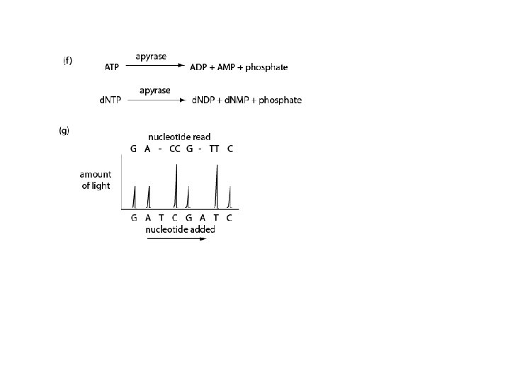
Pyrosequencing Advantages: • Very fast • Low cost per base • Large throughput; up to 40 megabases/epxeriment • No need for bacterial cloning (with its associated artifacts); this is especially helpful in metagenomics • High accuracy Disadvantages: • Short read lengths (soon to be extended to ~500 bp) • Difficulty sequencing homopolymers accurately Page 545

Page 546

Cycle termination sequencing (Solexa) (1) DNA is fragmented, adaptors are added (2) Single stranded DNA fragments attached to cell (3) DNA polymerase, d. NTPs for “bridge amplification” (4) Double-stranded bridges formed (5) Four labeled reversible terminators added (with primer and polymerase); one single terminator is added per cycle (6) Laser excitation to record the base (7) Reversible terminators are removed. All four labeled reversible terminators and polymerase are added for the next cycle. Page 547

Cycle termination sequencing (Solexa) Disadvantage: • Short read length (~36 bases; currently in 2009 ~75 bases) Advantages: • Very fast • Low cost per base • Large throughput; up to 1 gigabase/epxeriment • Short read length makes it appropriate for resequencing projects • No need for gel electrophoresis • High accuracy • All four bases are present at each cycle, with sequential addition of d. NTPs. This allows homopolymers to be accurately read.

Illumina sequencing technology in 12 steps Source: http: //www. illumina. com/downloads/SS_DNAsequencing. pdf

1. Prepare genomic DNA 2. Attach DNA to surface DNA 3. Bridge amplification adapters 4. Fragments become double stranded 5. Denature the doublestranded molecules 6. Complete amplification Randomly fragment genomic DNA and ligate adapters to both ends of the fragments

adapter DNA fragment 1. Prepare genomic DNA 2. Attach DNA to surface dense lawn of primers adapter 3. Bridge amplification 4. Fragments become double stranded 5. Denature the doublestranded molecules 6. Complete amplification Bind single-stranded fragments randomly to the inside surface of the flow cell channels

1. Prepare genomic DNA 2. Attach DNA to surface 3. Bridge amplification 4. Fragments become double stranded 5. Denature the doublestranded molecules 6. Complete amplification Add unlabeled nucleotides and enzyme to initiate solid-phase bridge amplification

1. Prepare genomic DNA 2. Attach DNA to surface Attached terminus free terminus Attached terminus 3. Bridge amplification 4. Fragments become double stranded 5. Denature the doublestranded molecules 6. Complete amplification The enzyme incorporates nucleotides to build double-stranded bridges on the solid-phase substrate

1. Prepare genomic DNA 2. Attach DNA to surface Attached 3. Bridge amplification 4. Fragments become double stranded 5. Denature the doublestranded molecules 6. Complete amplification Denaturation leaves singlestranded templates anchored to the substrate

1. Prepare genomic DNA 2. Attach DNA to surface 3. Bridge amplification 4. Fragments become double stranded Clusters 5. Denature the doublestranded molecules 6. Complete amplification Several million dense clusters of double-stranded DNA are generated in each channel of the flow cell

7. Determine first base 8. Image first base 9. Determine second base 10. Image second chemistry cycle 11. Sequencing over multiple chemistry cycles Laser The first sequencing cycle begins by adding four labeled reversible terminators, primers, and DNA polymerase 12. Align data

7. Determine first base 8. Image first base 9. Determine second base 10. Image second chemistry cycle 11. Sequencing over multiple chemistry cycles 12. Align data After laser excitation, the emitted fluorescence from each cluster is captured and the first base is identified

7. Determine first base 8. Image first base 9. Determine second base 10. Image second chemistry cycle 11. Sequencing over multiple chemistry cycles Laser The next cycle repeats the incorporation of four labeled reversible terminators, primers, and DNA polymerase 12. Align data

7. Determine first base 8. Image first base 9. Determine second base 10. Image second chemistry cycle 11. Sequencing over multiple chemistry cycles 12. Align data After laser excitation the image is captured as before, and the identity of the second base is recorded.

7. Determine first base 8. Image first base 9. Determine second base 10. Image second chemistry cycle 11. Sequencing over multiple chemistry cycles 12. Align data The sequencing cycles are repeated to determine the sequence of bases in a fragment, one base at a time.

Reference sequence 7. Determine first base 8. Image first base 9. Determine second base Unknown variant identified and called Known SNP called 10. Image second chemistry cycle 11. Sequencing over multiple chemistry cycles 12. Align data The data are aligned and compared to a reference, and sequencing differences are identified.

Outline of today’s lecture Introduction: 5 perspectives, history of life: time lines Genome-sequencing projects: chronology Genome analysis: criteria, resequencing, metagenomics DNA sequencing technologies: Sanger, 454, Solexa Process of genome sequencing: centers, repositories Genome annotation: features, prokaryotes, eukaryotes

Overview of genome analysis 20 Genome sequencing centers contributed to the public sequencing of the human genome. Many of these are listed at the Entrez genomes site. (Or see Table 19. 3, page 803. ) Page 548

Two approaches to genome sequencing Whole genome shotgun sequencing (Celera) Hierarchical shotgun sequencing (public consortium)

Two approaches to genome sequencing Whole Genome Shotgun (from the NCBI website) An approach used to decode an organism's genome by shredding it into smaller fragments of DNA which can be sequenced individually. The sequences of these fragments are then ordered, based on overlaps in the genetic code, and finally reassembled into the complete sequence. The 'whole genome shotgun' (WGS) method is applied to the entire genome all at once, while the 'hierarchical shotgun' method is applied to large, overlapping DNA fragments of known location in the genome. Page 548

Human genome project: strategies Whole genome shotgun sequencing (Celera) -- given the computational capacity, this approach is far faster than hierarchical shotgun sequencing -- the approach was validated using Drosophila

Two approaches to genome sequencing Hierarchical shotgun method Assemble contigs from various chromosomes, then sequence and assemble them. A contig is a set of overlapping clones or sequences from which a sequence can be obtained. The sequence may be draft or finished. A contig is thus a chromosome map showing the locations of those regions of a chromosome where contiguous DNA segments overlap. Contig maps are important because they provide the ability to study a complete, and often large segment of the genome by examining a series of overlapping clones which then provide an unbroken succession of information about that region. Page 548

Two approaches to genome sequencing Hierarchical shotgun sequencing (public consortium) -- 29, 000 BAC clones -- 4. 3 billion base pairs -- it is helpful to assign chromosomal loci to sequenced fragments, especially in light of the large amount of repetitive DNA in the genome -- individual chromosomes assigned to centers

Source: IHGSC (2001)

Source: IHGSC (2001)

Source: IHGSC (2001)

Sequenced-clone contigs are merged to form scaffolds of known order and orientation Source: IHGSC (2001) Fig. 19. 8 Page 804

When has a genome been fully sequenced? A typical goal is to obtain five to ten-fold coverage. Finished sequence: a clone insert is contiguously sequenced with high quality standard of error rate 0. 01%. There are usually no gaps in the sequence. Draft sequence: clone sequences may contain several regions separated by gaps. The true order and orientation of the pieces may not be known. Page 549

When has a genome been fully sequenced? Fold coverage 0. 25 0. 75 1 2 3 4 5 6 7 8 9 10 % sequenced 22 39 53 63 87. 5 95 98. 2 99. 4 99. 75 99. 91 99. 97 99. 995 Page 551

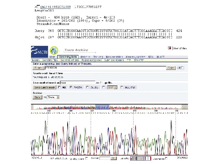
Trace repository for genome sequence data Raw data from many genome sequencing projects are stored at the trace archive at NCBI or EBI (~2 b traces). http: //trace. ensembl. org/ Page 552

Fig. 13. 12 Page 553

Fig. 13. 12 Page 553

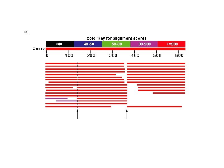
Blastn search of human trace archive with human RBP 4 (10/05): block-like structure of output reflects exons in the gene

Role of comparative genomics: utility of close versus distant comparisons Phylogenetic footprinting Phylogenetic shadowing Population shadowing Page 552

Fig. 13 Page 554

Outline of today’s lecture Introduction: 5 perspectives, history of life: time lines Genome-sequencing projects: chronology Genome analysis: criteria, resequencing, metagenomics DNA sequencing technologies: Sanger, 454, Solexa Process of genome sequencing: centers, repositories Genome annotation: features, prokaryotes, eukaryotes

Fig. 13. 14 Page 555

Genome annotation Information content in genomic DNA includes: -- nucleotide composition (GC content) -- repetitive DNA elements -- protein-coding genes, other genes These topics will be discussed later Page 555

GC content varies across genomes Bacteria Number of species in each GC class 10 5 Plants 5 Invertebrates 3 Vertebrates 10 5 20 30 40 50 60 70 GC content (%) 80 Fig. 13. 15 Page 556

Entrez Genomes at NCBI: GC content of 751 sequenced prokaryotic genomes GC content (%) number Updated 9/06

Next in the course Wednesday we discuss viruses (Chapter 14). Topics include HIV and the flu virus. Friday we turn to bacteria (lecture by Egbert Hoiczyk), then Monday discuss Chapter 15 (bacteria and archaea).