Creating the Vietoris Rips simplicial complex 0 Start

Creating the Vietoris Rips simplicial complex 0. ) Start by adding 0 -dimensional data points Note: we only need a definition of closeness between data points. The data points do not need to be actual points in Rn

Topology and Data. Gunnar Carlsson www. ams. org/journals/bull/2009 -46 -02/S 0273 -0979 -09 -01249 -X

http: //link. springer. com/article/10. 1007%2 Fs 00454 -004 -1146 -y

http: //link. springer. com/article/10. 1007/s 00454 -002 -2885 -2

U U U A filtered complex is an increasing sequence of simplicial complexes: C 0 C 1 C 2 … http: //link. springer. com/article/10. 1007%2 Fs 00454 -004 -1146 -y

U … C 05 U U C 20 U U {a, b, c} is in C 42 C 10 U U a, b is in C 00 U A filtered complex is an increasing sequence of simplicial complexes: C 0 C 1 C 2 … C 52 http: //link. springer. com/article/10. 1007%2 Fs 00454 -004 -1146 -y

3 2 1 0 C 2 C 1 C 0 0 H 0 = Z 0/B 0 = (kernel of 0)/ (image of null space of M 0 = column space of M 1 Rank H 0 = Rank Z 0 – Rank B 0 1)

3 C 2 2 C 1 1 C 0 0 0 H 0 = Z 0/B 0 = (kernel of 0)/ (image of null space of M 0 = column space of M 1 Rank H 0 = Rank Z 0 – Rank B 0 1)

0 0 0 http: //link. springer. com/article/10. 1007%2 Fs 00454 -004 -1146 -y

0 0 0 http: //link. springer. com/article/10. 1007%2 Fs 00454 -004 -1146 -y

0 0 0 H 0 = Z 0/B 0 = (kernel of 0)/ (image of 1) http: //link. springer. com/article/10. 1007%2 Fs 00454 -004 -1146 -y

0 0 0 i, 0 H 0 = i Z 0 / i B 0 0 = (kernel of 0)/ (image of 1) http: //link. springer. com/article/10. 1007%2 Fs 00454 -004 -1146 -y

0 0 0 0, 1 H 0 = 0 0+1 Z 0 / ( B 0 U 0 0 Z 0 ) http: //link. springer. com/article/10. 1007%2 Fs 00454 -004 -1146 -y

0 0 0 0, 2 H 0 = 0 0+2 Z 0 / ( B 0 U 0 0 Z 0 ) http: //link. springer. com/article/10. 1007%2 Fs 00454 -004 -1146 -y

0 0 0 i, 1 H 0 = i i+1 Z 0 / ( B 0 U 0 i Z 0 ) http: //link. springer. com/article/10. 1007%2 Fs 00454 -004 -1146 -y

= i i+2 Z 0 / ( B 0 U i, 2 H 0 i Z 0 ) http: //link. springer. com/article/10. 1007%2 Fs 00454 -004 -1146 -y

U p-persistent kth homology group: i, p i i+p Hk = Z k / ( B k i Zk ) http: //link. springer. com/article/10. 1007%2 Fs 00454 -004 -1146 -y

o 2 o 1 C 2 C 1 C 0 H 1 = Z 1/B 1 = (kernel of o 1 )/ (image of o 2 ) null space of M 1 = column space of M 2 <e 1 + e 2 + e 3, e 4 + e 5 + e 6> = <e 4 + e 5 + e 6> Rank H 1 = Rank Z 1 – Rank B 1 = 2 – 1 = 1

Topological Persistence and Simplification, 2002 Figure from: Computing Persistent Homology, 2005 Let s be a k-simplex s is a positive simplex if it creates a cycle when it enters. s is a negative simplex if it destroys a cycle when it enters. http: //link. springer. com/article/10. 1007%2 Fs 00454 -004 -1146 -y

Computing Persistent Homology by Afra Zomorodian, Gunnar Carlsson 0 0 1 1 2 2 3 4 a b c d ab bc cd ad ac abc acd 0 1 2 3 4 5 6 7 8 9 5 10 http: //link. springer. com/article/10. 1007%2 Fs 00454 -004 -1146 -y

Computing Persistent Homology by Afra Zomorodian, Gunnar Carlsson 0 0 1 1 2 2 3 4 5 + + - - - + + - - a b c d ab bc cd ad ac abc acd 0 1 2 3 4 5 6 7 8 4 5 6 10 9 ad ac a, b b, c c, d 9 10 http: //link. springer. com/article/10. 1007%2 Fs 00454 -004 -1146 -y

0 0 1 1 2 2 3 4 5 + + - - - + + - - a b c d ab bc cd ad ac abc acd 0 1 2 3 4 5 6 7 8 4 5 6 10 9 ad ac a, b b, c c, d a 0 1 3 b 0 c 1 d 1 ab 1 bc 1 cd 2 ad 2 9 10 ac 3 abc 4 acd 5

[ a 0 1 3 b 0 [ c 1 [ ) d 1 ) ) [ ab 1 bc 1 cd 2 ad 2 [ ) ) ac 3 abc 4 acd 5

[ a 0 1 3 b 0 [ c 1 [ ) d 1 ) ) [ ab 1 bc 1 cd 2 ad 2 [ ) ) ac 3 abc 4 acd 5

a 0 b 0 c 1 d 1 ab 1 bc 1 cd 2 ac 3 abc 4 acd 5 1 3 [ t 0 1 3 [ ) t 1 ) [ [ t 2 t 3 ) t 4 ) t 5

[ a 0 b 0 [ c 1 [ ) d 1 ) ) [ [ ab 1 bc 1 cd 2 ad 2 ) ) ac 3 abc 4 acd 5 1 3 [ t 0 1 3 [ ) t 1 ) [ [ t 2 t 3 ) t 4 ) t 5

Topological Persistence and Simplification: link. springer. com/article/10. 1007/s 00454 -002 -2885 -2

Topological Persistence and Simplification: link. springer. com/article/10. 1007/s 00454 -002 -2885 -2

Topological Persistence and Simplification: link. springer. com/article/10. 1007/s 00454 -002 -2885 -2

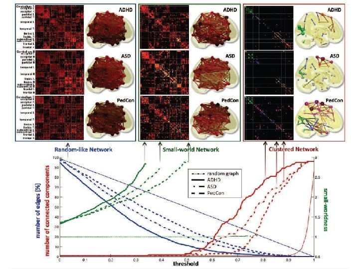
Discriminative persistent homology of brain networks, 2011 Hyekyoung Lee Chung, M. K. ; Hyejin Kang; Bung-Nyun Kim; Dong Soo Lee Constructing functional brain networks with 97 regions of interest (ROIs) extracted from FDG-PET data for 24 attention-deficit hyperactivity disorder (ADHD), 26 autism spectrum disorder (ASD) and 11 pediatric control (Ped. Con). Data = measurement fj taken at region j Graph: 97 vertices representing 97 regions of interest edge exists between two vertices i, j if correlation between fj and fj ≥ threshold How to choose threshold? Don’t, instead use persistent homology

Vertices = Regions of Interest Create Rips complex by growing epsilon balls (i. e. decreasing threshold) where distance between two vertices is given by where fi = measurement at location i

Discriminative persistent homology of brain networks, 2011 Hyekyoung Lee Chung, M. K. ; Hyejin Kang; Bung-Nyun Kim; Dong Soo Lee Constructing functional brain networks with 97 regions of interest (ROIs) extracted from FDG-PET data for 24 attention-deficit hyperactivity disorder (ADHD), 26 autism spectrum disorder (ASD) and 11 pediatric control (Ped. Con). Data = measurement fj taken at region j Graph: 97 vertices representing 97 regions of interest edge exists between two vertices i, j if correlation between fj and fj ≥ threshold How to choose threshold? Don’t, instead use persistent homology

2012 Ignoble Prize The Ig Nobel Prizes honor achievements that make people LAUGH, and then THINK. http: //www. improbable. com/ig/ Activated f. MRI of dead salmon The salmon was shown images of people in social situations, either socially inclusive situations or socially exclusive situations. The salmon was asked to respond, saying how the person in the situation must be feeling. http: //blogs. scientificamerican. com/sc icurious-brain/2012/09/25/ignobelprize-in-neuroscience-the-deadsalmon-study/ compared to other voxels

© 2008 I. K. Darcy. All rights reserved

http: //www. ploscompbiol. org/article/info%3 Adoi%2 F 10. 1371%2 Fjournal. pcbi. 1000205 2008 First paper to use only the spiking activity of place cells to determine the topology (and geometry) of the environment using homology (and graphs).

Edvard Moser May-Britt Moser John O’Keefe http: //www. nature. com/news/nobel-prize-for-decoding-brain-s-sense-of-place-1. 16093

http: //www. nature. com/news/neuroscience-brains-ofnorway-1. 16079 May-Britt Moser Edvard Moser John O’Keefe http: //www. nature. com/news/nobel-prize-for-decoding-brain-s-sense-of-place-1. 16093

place cells = neurons in the hippocampus that are involved in spatial navigation http: //en. wikipedia. org/wiki/File: Gray 739 -emphasizing-hippocampus. png http: //en. wikipedia. org/wiki/File: Hippocampus. gif http: //en. wikipedia. org/wiki/File: Hippocampal-pyramidal-cell. png

http: //www. nytimes. com/2014/10/07/science /nobel-prize-medicine. html

http: //www. ploscompbiol. org/article/info%3 Adoi%2 F 10. 1371%2 Fjournal. pcbi. 1002581

http: //www. ntnu. edu/kavli/research/grid-cell-data

http: //www. ploscompbiol. org/article/info%3 Adoi%2 F 10. 1371%2 Fjournal. pcbi. 1000205 2008 First paper to use only the spiking activity of place cells to determine the topology (and geometry) of the environment using homology (and graphs).

Place field = region in space where the firing rates are significantly above baseline place cells = neurons in the hippocampus that are involved in spatial navigation http: //www. ploscompbiol. org/article/info%3 Adoi%2 F 10. 1371%2 Fjournal. pcbi. 1002581

How can the brain understand the spatial environment based only on action potentials (spikes) of place cells? http: //upload. wikimedia. org/wikipedia/en/5/5 e/Place_Cell_Spiking_Activity_Example. png

Time Cycles

Time Cycles

Time Cycles

Time Cycles

Time Cycles

Time Cycles

Time Cycles

Time Cycles

Time Cycles

Time Cycles

Time Cycles

Time Cycles

Time Cycles

How can the brain understand the spatial environment based only on action potentials (spikes) of place cells? http: //upload. wikimedia. org/wikipedia/en/5/5 e/Place_Cell_Spiking_Activity_Example. png

Place field = region in space where the firing rates are significantly above baseline http: //www. ploscompbiol. org/article/info%3 Adoi%2 F 10. 1371%2 Fjournal. pcbi. 1000205

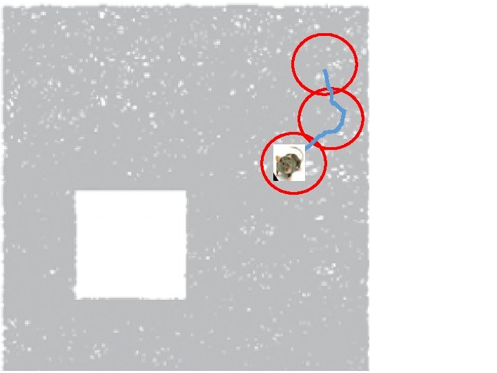
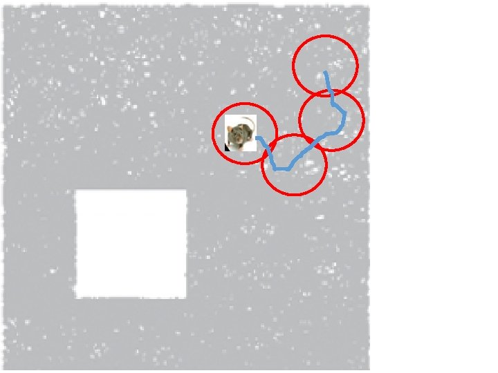
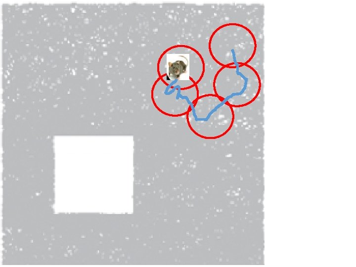
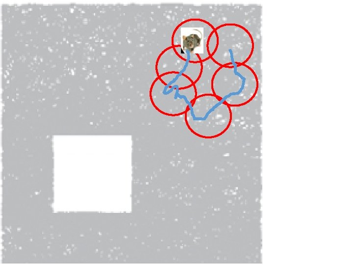
Idea: Can recover the topology of the space traversed by the mouse by looking only at the spiking activity of place cells. http: //www. ploscompbiol. org/article/info%3 Adoi%2 F 10. 1371%2 Fjournal. pcbi. 1000205

Creating a simplicial complex

Creating a simplicial complex 1. ) Adding 1 -dimensional edges (1 -simplices) Add an edge between data points that are “close”

Creating the Čech simplicial complex 1. ) B 1 … Bk+1 ≠ 0⁄ , create k-simplex {v 1, . . . , vk+1}. U U

Creating the Čech simplicial complex 1. ) B 1 … Bk+1 ≠ 0⁄ , create k-simplex {v 1, . . . , vk+1}. U U

Consider X an arbitrary topological space. Let V = {Vi | i = 1, …, n } where Vi X, The nerve of V = N(V) where The k -simplices of N(V) = nonempty intersections of k +1 distinct elements of V. For example, Vertices = elements of V Edges = pairs in V which intersect nontrivially. Triangles = triples in V which intersect nontrivially. http: //www. math. upenn. edu/~ghrist/EATchapter 2. pdf

Consider X an arbitrary topological space. Čech complex = Let V = {Vi | i = 1, …, n } where Vi Mathematical X, nerve, not biological nerve The nerve of V = N(V) where The k -simplices of N(V) = nonempty intersections of k +1 distinct elements of V. For example, Vertices = elements of V Edges = pairs in V which intersect nontrivially. Triangles = triples in V which intersect nontrivially. http: //www. math. upenn. edu/~ghrist/EATchapter 2. pdf

Creating the Čech simplicial complex 1. ) B 1 … Bk+1 ≠ 0⁄ , create k-simplex {v 1, . . . , vk+1}. U U

Mathematical Nerve Lemma: If V is a finite collection of subsets of X with all non-empty intersections of subcollections of V contractible, then N(V) is homotopic to the union of elements of V. http: //www. math. upenn. edu/~ghrist/EATchapter 2. pdf

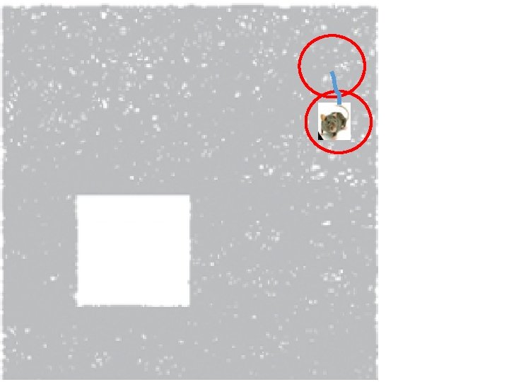
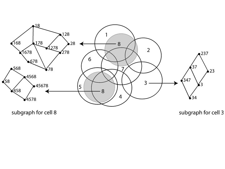
Idea: Can recover the topology of the space traversed by the mouse by looking only at the spiking activity of place cells. Vertices = place cells Add simplex if place cells co-fare within a specified time period http: //www. ploscompbiol. org/article/info%3 Adoi%2 F 10. 1371%2 Fjournal. pcbi. 1000205

Cell group = collection of place cells that co-fire within a specified time period (above a specified threshold). Simplices correspond to cell groups. dimension of simplex = number of place cells in cell group - 1 http: //www. ploscompbiol. org/article/info%3 Adoi%2 F 10. 1371%2 Fjournal. pcbi. 1000205

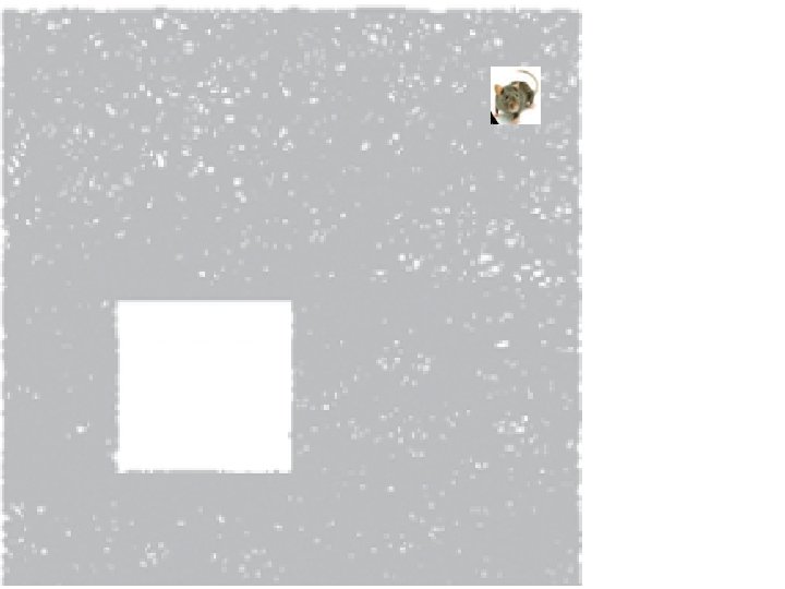
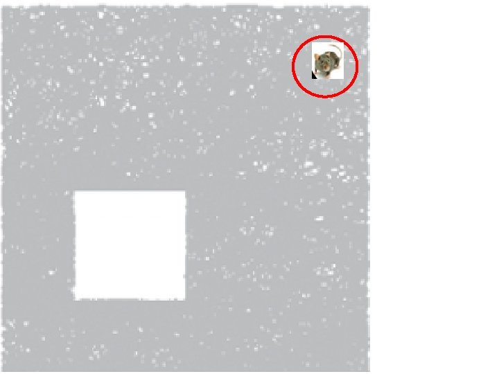
Idea: Can recover the topology of the space traversed by the mouse by looking only at the spiking activity of place cells. Proof of concept: Data obtained via computer simulations of mouse trajectories using biologically relevant parameters. http: //www. ploscompbiol. org/article/info%3 Adoi%2 F 10. 1371%2 Fjournal. pcbi. 1000205

a smoothed random-walk trajectory was generated, with speed = 0. 1 L/s, which was constrained to ‘‘bounce’’ off boundaries and stay within the environment. The total duration of each simulated trajectory was 50 minutes. http: //www. ploscompbiol. org/article/info%3 Adoi%2 F 10. 1371%2 Fjournal. pcbi. 1000205

For each of 300 trials, N= 70 place fields were generated as disks of radii 0. 1 L to 0. 15 L, with radii and centers chosen uniformly at random. Centers were chosen initially uniformly at random from uncovered space. Once all space covered, remaining centers chosen at random. http: //www. ploscompbiol. org/article/info%3 Adoi%2 F 10. 1371%2 Fjournal. pcbi. 1000205

For each place cell in each trial, an average firing rate was chosen uniformly at random from the interval 2– 3 Hz. A spike train was generated from the trajectory and corresponding place field as an inhomogeneous Poisson process with constant rate when the trajectory passed inside the place field, and zero outside, so that the overall firing rate was preserved.

Add noise. r% spikes were deleted from the spike train, and then added back to the spike train at random times, irrespective of position along trajectory, so as to preserve overall firing rate. Control : ‘Shuffled’ data sets were constructed by randomly choosing cells from each of the five environments, and pooling them together to yield population spiking activity that did not come from a single environment.

Assumptions about Place Fields (1) Place fields are omni-directional I. e. direction does not affect the firing rate. http: //www. ploscompbiol. org/article/info%3 Adoi%2 F 10. 1371%2 Fjournal. pcbi. 1000205

Assumptions about Place Fields (1) Place fields are omni-directional Correct assumption in open field. Not correct in linear track. Place cells can also encode angles and directions http: //www. ploscompbiol. org/article/info%3 Adoi%2 F 10. 1371%2 Fjournal. pcbi. 1000205

Assumptions about Place Fields (1) Place fields are omni-directional (2) Place fields have been previously formed and are stable. http: //www. ploscompbiol. org/article/info%3 Adoi%2 F 10. 1371%2 Fjournal. pcbi. 1000205

Assumptions about Place Fields (1) Place fields are omni-directional (2) Place fields have been previously formed and are stable. Note: the hippocampus can undergo rapid context dependent remapping. http: //www. ploscompbiol. org/article/info%3 Adoi%2 F 10. 1371%2 Fjournal. pcbi. 1000205

Assumptions about Place Fields (1) Place fields are omni-directional (2) Place fields have been previously formed and are stable. Note: the hippocampus can undergo rapid context dependent remapping. http: //www. ploscompbiol. org/article/info%3 Adoi%2 F 10. 1371%2 Fjournal. pcbi. 1000205

Assumptions about Place Fields (1) Place fields are omni-directional (2) Place fields have been previously formed and are stable. Note: the hippocampus can undergo rapid context dependent remapping. http: //www. ploscompbiol. org/article/info%3 Adoi%2 F 10. 1371%2 Fjournal. pcbi. 1000205

Assumptions about Place Fields (1) Place fields are omni-directional (2) Place fields have been previously formed and are stable. Note: the hippocampus can undergo rapid context dependent remapping. Nature 2002, Long-term plasticity in hippocampal place-cell representation of environmental geometry, Colin Lever, Tom Wills, Francesca Cacucci, Neil Burgess, John O'Keefe http: //www. nature. com/nature/journal/v 416/n 6876/fig_tab/416090 a_F 2. html

Remodeling: the hippocampus can undergo rapid context dependent remapping. http: //arxiv. org/abs/q-bio/0702052

Assumptions about Place Fields (1) Place fields are omni-directional (2) Place fields have been previously formed and are stable. (3) The collection of place fields corresponding to observed cells covers the entire traversed environment. I. e. , the trajectory must be dense enough to sample the majority of cell groups. http: //www. ploscompbiol. org/article/info%3 Adoi%2 F 10. 1371%2 Fjournal. pcbi. 1000205

Assumptions about Place Fields (1) Place fields are omni-directional (2) Place fields have been previously formed and are stable. (3) The collection of place fields corresponding to observed cells covers the entire traversed environment. Biologically: place cells multiply cover the environment. http: //www. ploscompbiol. org/article/info%3 Adoi%2 F 10. 1371%2 Fjournal. pcbi. 1000205

Assumptions about Place Fields (1) Place fields are omni-directional (2) Place fields have been previously formed and are stable. (3) The collection of place fields corresponding to observed cells covers the entire traversed environment. For accurate computation of the nth homology group Hn, we need up to (n+1)-fold intersections to be detectable via cell groups. http: //www. ploscompbiol. org/article/info%3 Adoi%2 F 10. 1371%2 Fjournal. pcbi. 1000205

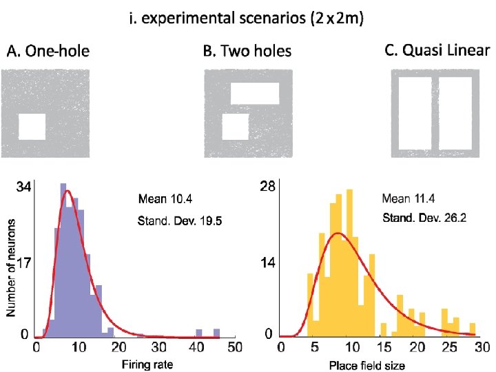
Assumptions about Place Fields (1) Place fields are omni-directional (2) Place fields have been previously formed and are stable. (3) The collection of place fields corresponding to observed cells covers the entire traversed environment. (4) The holes/obstacles are larger than the diameters of place fields. http: //www. ploscompbiol. org/article/info%3 Adoi%2 F 10. 1371%2 Fjournal. pcbi. 1000205

Assumptions about Place Fields (5) Each (connected) component field of a single or multipeaked place field is convex. (6) Background activity is low compared to the firing inside the place fields. (7) Place fields are roughly circular and have similar sizes, as is typical in dorsal hippocampus [41, 42]. http: //www. ploscompbiol. org/article/info%3 Adoi%2 F 10. 1371%2 Fjournal. pcbi. 1000205

For each place cell in each trial, an average firing rate was chosen uniformly at random from the interval 2– 3 Hz. A spike train was generated from the trajectory and corresponding place field as an inhomogeneous Poisson process with constant rate when the trajectory passed inside the place field, and zero outside, so that the overall firing rate was preserved. Noise added.

Cell group = collection of place cells that co-fire within a specified time period (above a specified threshold). Simplices correspond to cell groups. dimension of simplex = number of place cells in cell group - 1 http: //www. ploscompbiol. org/article/info%3 Adoi%2 F 10. 1371%2 Fjournal. pcbi. 1000205

Homology calculated via the GAP software package: http: //www. cis. ude l. edu/linbox/gap. ht ml Simplices correspond to cell groups. dimension of simplex = number of place cells in cell group - 1 http: //www. ploscompbiol. org/article/info%3 Adoi%2 F 10. 1371%2 Fjournal. pcbi. 1000205

Recovering the topology Trial is correct if Hi correct for i = 0, 1, 2, 3, 4. http: //www. ploscompbiol. org/article/info%3 Adoi%2 F 10. 1371%2 Fjournal. pcbi. 1000205

Geometry? ? ?

http: //www. ploscompbiol. org/article/info%3 Adoi%2 F 10. 1371%2 Fjournal. pcbi. 1000205 First paper to use only the spiking activity of place cells to determine the topology (and geometry) of the environment using homology (and graphs).

http: //www. ploscompbiol. org/article/info%3 Adoi%2 F 10. 1371%2 Fjournal. pcbi. 1000205

m 1 = 1 mk = 1 – p √(k-1)/N where N = number of cells. http: //www. ploscompbiol. org/article/info%3 Adoi%2 F 10. 1371%2 Fjournal. pcbi. 1000205

Normalize distance so mean pairwise distances same for both simulated and calculated data. http: //www. ploscompbiol. org/article/info%3 Adoi%2 F 10. 1371%2 Fjournal. pcbi. 1000205

http: //www. ploscompbiol. org/article/info%3 Adoi%2 F 10. 1371%2 Fjournal. pcbi. 1000205

Normalize distance so mean pairwise distances same for both simulated and calculated data. http: //www. ploscompbiol. org/article/info%3 Adoi%2 F 10. 1371%2 Fjournal. pcbi. 1000205

http: //www. ploscompbiol. org/article/info%3 Adoi%2 F 10. 1371%2 Fjournal. pcbi. 1000205

Multipeaked place fields http: //www. ploscompbiol. org/article/info%3 Adoi%2 F 10. 1371%2 Fjournal. pcbi. 1000205

http: //www. ploscompbiol. org/article/info%3 Adoi%2 F 10. 1371%2 Fjournal. pcbi. 1000205

http: //www. ploscompbiol. org/article/info%3 Adoi%2 F 10. 1371%2 Fjournal. pcbi. 1002581 2012

2012

2012

Data obtained via computer simulations

http: //www. ntnu. edu/kavli/research/grid-cell-data

Note the above examples use the Čech complex to determine the topology of the mouse environment. But often in topological data analysis for computational efficiency, one uses the Rips complex instead of the Čech complex. Unfortunately there is no nerve lemma for the Rips complex.

Creating the Vietoris Rips simplicial complex 0. ) Start by adding 0 -dimensional data points Note: we only need a definition of closeness between data points. The data points do not need to be actual points in Rn

Creating the Vietoris Rips simplicial complex Step 0. ) Start by adding data points = 0 -dimensional vertices (0 -simplices)

Creating the Vietoris Rips simplicial complex 1. ) Adding 1 -dimensional edges (1 -simplices) Add an edge between data points that are “close”

Creating the Vietoris Rips simplicial complex 2. ) Add all possible simplices of dimensional > 1.

Vietoris Rips complex = flag complex = clique complex 2. ) Add all possible simplices of dimensional > 1.

Creating the Čech simplicial complex 1. ) B 1 … Bk+1 ≠ 0⁄ , create k-simplex {v 1, . . . , vk+1}. U U

Creating the Čech simplicial complex 1. ) B 1 … Bk+1 ≠ 0⁄ , create k-simplex {v 1, . . . , vk+1}. U U