INEL 5995 Weather Radar Network Topics Prof Hctor


 Networks' microwave radio systems enable transmission connections in places where")

 ¢ The situation is very different in a")
 ¢ The cross-layer protocol design of wireless networks")

")


 ¢ 1 - Identificar características y requisitos")


.")


 ¢ 2 - Identificar rangos de frecuencia")


. Ver documento en Web. Ct,")

 ¢ 3 - Identificar alternativas de transmisión")


 y diferentes mecanismos")
 ¢ 4 - Analizar preliminarmente las posibles")


 ¢ 5 - Identificar las características principales")
 Point 2: UPR-Mayagüez (18.")
 ¢ 6 - Seleccionar una ruta y")
 Point 2: UPR-Mayagüez (18.")
 Point 2: UPR-Mayagüez (18.")


 ¢ 7 - Usar un software package")


 Point 2: UPR-Mayagüez (18.")


")


, power")


 ¢ 8 - Repetir el paso anterior")
 Pt db =")

 True North Azimuth =")
 True North Azimuth = 4.")
: Tx Power=10 w (40 d. Bm), Gt=5 d. Bi (2. 85 d.")
 ¢ ¢")
 ¢ 9 - Hacer pruebas de propagación")

 ¢ 10 - Usar Gaussian distribution, y")
 ¢ 11 - Usar Matlab para comparar")
 Name")
")
 ¢ ¢ 12 - Dimensionar de nuevo")
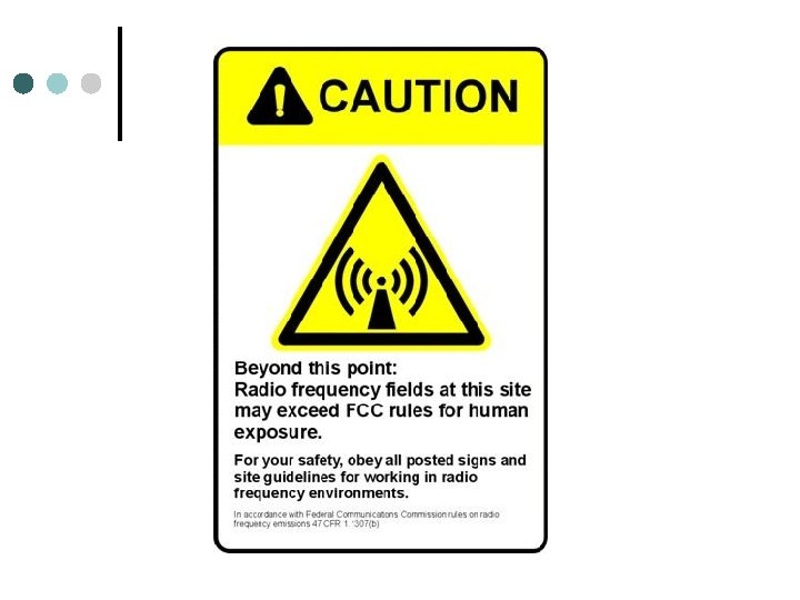
 Guidelines for human exposure limits. Human Exposure")


 Material Energía Ionizante Hidrógeno 13. 6 e.")


 Maximum Limits of Average Power from Man-made sources 106")
 AM/FM Transmitter 5 -50 k. W)")

 ¢")


 • l ~ = The Body In this")


 ¢ 12 - Identificar proveedores de los")
")


 Elaborar documentos: Lista de equipos, antenas, cables,")

 Noise Figure Measurement Setup: Spectrum Analyzer DUT RF Noise Source Pre")


")


- Slides: 149
INEL 5995 Weather Radar Network Topics Prof. Héctor Monroy hmonroy@ece. uprm. edu Of. S-413
¿Qué se estudia en esta parte del curso? Cómo se transmiten los datos que toman los radares (tales como los de CASA), desde el sitio de cada radar hasta un centro de recolección de datos
This slide is taken from a presentation by Brian C. Donovan, Ph. D Student UMass, Project Manager April 27, 2004 Puerto Rico Student Test Bed (IP-3)
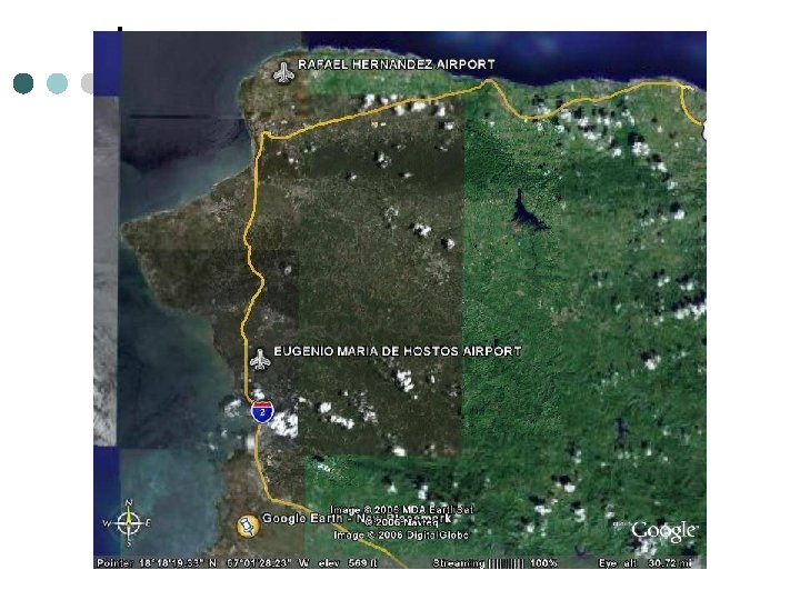
Location Possibilities. Slide taken from a presentation by Brian C. Donovan, Ph. D Student UMass, Project Manager April 27, 2004 Mayagüez - Aguadilla 31. 3 km Mayagüez – Arecibo 50. 7 km Aguadilla – Arecibo 42. 0 km Node Spacing Mayagüez - Aguadilla 31. 3 km Mayagüez – Isabela 35. 0 km Aguadilla – Isabela 12. 5 km Node Spacing
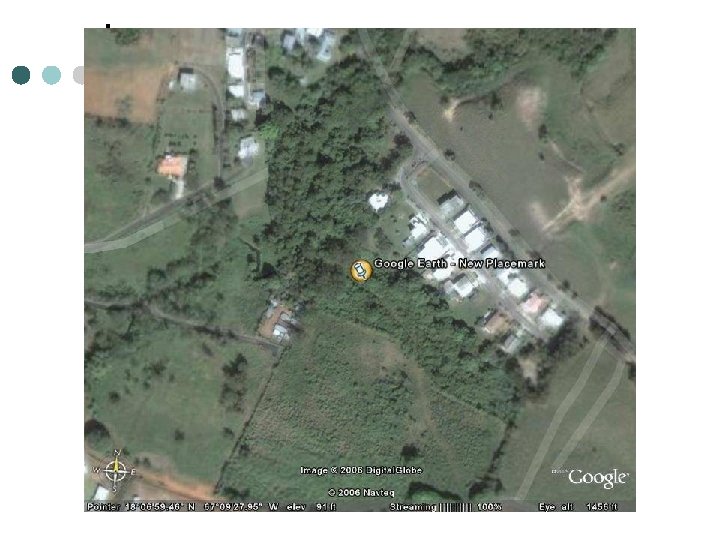
Ejemplo: Cómo traer al RUM los datos colectados por un radar que se va a instalar próximamente en la Finca la Montaña, Aguadilla, en el sitio localizado en 18° 28. 465’ N, 67° 07. 267’ W
Proposed Location This slide is taken from a presentation by José Maeso and Jorge M. Trabal July 2004 UPRM Aguadilla (259’ over sea level)
Preguntas a responder inicialmente: ¿Qué vamos a transmitir? ¢ ¿Cómo lo vamos a transmitir? ¢ ¿Qué mecanismo de propagación debemos usar? Luego de responder lo anterior, se ataca el problema de cómo diseñar el sistema para transmitir los datos a un centro de recolección. ¢
Alternativas para enviar los datos desde los radares al RUM: Poner datos en Removable Disk y mandarlos con alguien (bueno…si no hay prisa). ¢ Mandarlos vía Wired Network ¢ Mandarlos vía Wireless Network (si son varios radares, podría ser conveniente tener un centro de recolección, y de ahí enviar todos los datos al RUM, todo vía wireless). ¢
Conviene sabor algo sobre Types of Networks: Private Networks ¢ http: //www. stratexnet. com/products/pri vate_networks/ Mobile Networks ¢ http: //www. stratexnet. com/products/m obile_networks/ Fixed Networks ¢ http: //www. stratexnet. com/products/fix ed_networks/
Tomado de los websites anteriores PRIVATE NETWORKS Private networks employ a variety of applications. Utility communications networks are a large user of microwave throughout the world, connecting oil and gas installations, pipelines, and even drilling platforms at sea. Campus-based university, health authority, and government networks are also an ideal application for microwave, providing connectivity between buildings that are co-located or distributed throughout a city or metropolitan area. These networks are self-contained, carrying PABX voice and LAN/WAN data traffic. National and regional TV networks also use microwave for contribution/distribution links between studios and broadcasting sites that are typically located on remote mountaintop locations where cable connectivity is impractical.
MOBILE NETWORKS Microwave radio is the medium of choice for mobile infrastructures worldwide, providing a compelling backhaul solution for operators of Mobile Cellular Networks. The demand for microwave, driven in the 1990's by the expansion of GSM in Europe, is now set to be eclipsed by the 2002 rollout of 3 G mobile networks. 3 G technology combines the typical benefits of microwave radio, including cost-effective and rapid deployment, easy capacity upgrade, and minimal operational costs, with the ability for operators to establish and maintain their own transmission links, instead of leasing expensive circuits from local fixedline operators.
FIXED NETWORS A significant number of businesses remain disconnected from the information superhighway because they lack available wired broadband infrastructure. Wireless provides the perfect medium for breaking down the barriers of this "digital divide, " whether in a city center or a remote rural community.
FIXED NETWORKS (cont. ) Networks' microwave radio systems enable transmission connections in places where fiber cannot reach, where build is prohibitively expensive, when local authorities refuse or inhibit right-of-way for cable deployments, as a wireless backup for critical fiber links, or for dedicated wireless lastmile access.
Wired and wireless networks ¢ Wired networks typically satisfy diverse requirements of different applications using a single protocol. This means the most stringent requirements for all applications must be met simultaneously. Wired networks may have data rates of Gbps and BERs of 10 -12. ¢ Currently exists a tremendous infrastructure of wired networks: the telephone system, the Internet, fiber optic, cables. This infrastructure could be used to connect wireless systems together into a global network. ¢ Wired networks are mostly designed according to a layered approach, whereby protocols associated with different layers of the system operation are designed in isolation, with baseline mechanisms to interface between layers. ¢ The layered approach (layering methodology) of wired networks reduces complexity and facilitates modularity and standardization, but it also leads to inefficiency and performance loss, due to the lack of a global design optimization.
Wired and wireless networks (cont. 1) ¢ The situation is very different in a wireless network due to the nature of radiopropagation and broadcasting. ¢ The wireless network must be able to locate a given user wherever it is among billions of globally distributed terminals (if it is a mobile terminal, the system must route the signal to a user as it moves at a certain speed). ¢ The layers in a wireless system include: the link or physical layer (handles bit transmission over the communications medium); the access layer (handles shared access to the communications medium); the network and transport layers (which route data across the network and ensure end-to-end connectivity and data delivery); and the application layer (dictates the end-to-end data rates and delay constraints associated with the application). ¢ Wireless networks required integrated and adaptive protocols at all layers, from the link layer to the application layer.
Wired and wireless networks (cont. 2) ¢ The cross-layer protocol design of wireless networks requires interdisciplinary expertise in communications, signal processing, and network theory and design. ¢ Wireless networks, at least in the near future, will continue to be fragmented, with different protocols tailored to support the requirements of different applications. Wireless networks have much lower data rates and higher BERs. ¢ Interfacing between wired and wireless networks with different performance capabilities is a difficult problem.
Since different wireless applications have different requirements ¢ There are many ways to segment this topic into different applications, systems, and coverage regions. ¢ This has resulted in considerable fragmentation in the industry. ¢ There are many different products, standards, and services being offered or proposed. ¢ See the 55 pages New American Public Knowledge (by Kevin Werbach).
Lectura recomendada (cultura general sobre telecomunicaciones, para el gran público)
Conviene también leer algo sobre Planning Microwave Links. Ver, por ejemplo, http: //www. stratexnet. com/about_us/our_te chnology/files/planning_article/taju 95. html Ver también el website
Etapas de un diseño, desde el punto de vista de Comunicaciones: Circuitos y Antenas ( !OJO! Es diferente si se ve desde el punto de vista de Signal Processing o de Computer Science) ¢ 1 - Identificar características y requisitos de los datos a ser transmitidos (R, B, BER, SNR, SINR, etc. ). ¢ 2 - Identificar rangos de frecuencia que se pueden usar (Recomendaciones y Normas ITU-R, FCC, IEEE). ¢ 3 - Identificar posibles alternativas de transmisión, y escoger la mejor (enfatizaremos LOS, y algún stándard IEEE 802. 11).
Etapas de un diseño, desde el punto de vista de Comunicaciones: Circuitos y Antenas (no de Signal Processing ni Computer Science) (cont. 1) ¢ 4 - Analizar preliminarmente las posibles rutas de propagación (usar Google Earth, USGS). ¢ 5 - Identificar las características generales de las posibles rutas de propagación (podrían usarse, por ejemplo, mapas de 1: 25, 000 de USGS en el Web). ¢ 6 - Seleccionar la ruta más viable y obtener la base de datos topográficos (Digital Elevation Models, USGS).
Etapas de un diseño, desde el punto de vista de Comunicaciones: Circuitos y Antenas (no de Signal Processing ni Computer Science) (cont. 2) ¢ 7 - Usar un software package (Radio Mobile, Radiosoft Comstudy, Planner, etc. ) para analizar rutas y escoger alturas de antenas según requisitos de Zonas de Fresnel, reflexiones, etc. ¢ 8 - Repetir paso anterior con diferentes condiciones atmosféricas (K = 5/3, 4/3, 1, 2/3). Escoger ruta y dismensionar preliminarmente el sistema (Tx, Rx, antenas, líneas, etc. ). ¢ 9 - Hacer pruebas de propagación (si hay los medios para tomar muestras), o usar Matlab para simular una señal recibida con los parámetros escogidos preliminarmente en el paso anterior.
Etapas de un diseño, desde el punto de vista de Comunicaciones: Circuitos y Antenas (no de Signal Processing ni Computer Science) (cont. 3) ¢ 10 - Usar Gaussian distribution, y determinar mean, std, etc. de la señal simulada (o muestra recibida) para adecuar el sistema a la confiabilidad de operación especificada. ¢ 11 - Usar Matlab para confirmar algunos resultados, haciendo el perfil topográfico de la ruta con la base de datos y simulando niveles de señal, de acuerdo al paso anterior. ¢ 12 - Dimensionar de nuevo el sistema. !Tener en cuenta cálculos de SAR, aunque se use baja potencia!
Etapas de un diseño, desde el punto de vista de Comunicaciones: Circuitos y Antenas (no de Signal Processing ni Computer Science) (cont. 4) ¢ 13 - Identificar proveedores de los equipos y componentes apropiados y hacer selección final del sistema, ajustado a los requisitos del diseño y a las Recomendaciones y Normas de ITU-R, FCC, IEEE, OSHA. ¢ 14 - Hacer lista de equipos, antenas, torres, cables…y componentes necesarios para instalar el sistema. ¢ 15 - Elaborar documento explicativo sobre las mediciones necesarias para optimizar el funcionamiento del sistema. ¢ 16 - Hacer un Resumen Ejecutivo.
Detalles de las Etapas de Diseño (1) ¢ 1 - Identificar características y requisitos de los datos a ser transmistidos ( R, B, BER, SNR, SINR, etc. ).
-Application (Voice, sensing, file transfer, video teleconferencing, distributing control, paging and short messaging, Internet access, Web browsing, etc). -Systems (cellular telephone, wireless LANs, wide area wireless data, satellite, ad hoc wireless netwoks). -Coverage (building, city, regional, global). See p. 5 Wireless Comm. , A. Goldsmith, Cambridge, 2005.
Requirements for different applications make it difficult to build one system that can satisfy all requirements simultaneously. Voice systems: ¢ ¢ ¢ Have low data-rate requirements (around 20 kbps). Can tolerate high probability of bit error (BERs of around 10 -3), but The total delay must be less than 100 ms or else it becomes noticeable to the end user (wired telephones have delay constraint of ≈30 ms, cellular phones ≈100 ms, voice over the Internet relaxes the constraint even further).
Data systems: ¢ ¢ ¢ Typically require much higher data rates (1 -100 Mbps). Very small BERs (10 -10 or less, and all bits received in error must be retransmitted). Do not have a fixed delay requirement.
Real-time video systems: ¢ Have high data-rate requirements coupled with the same delay constraints as voice systems. Paging and short messaging: ¢ Have very low data-rate requirements and no hard delay constraints.
Si queremos comunicar dos puntos del Oeste de PR…
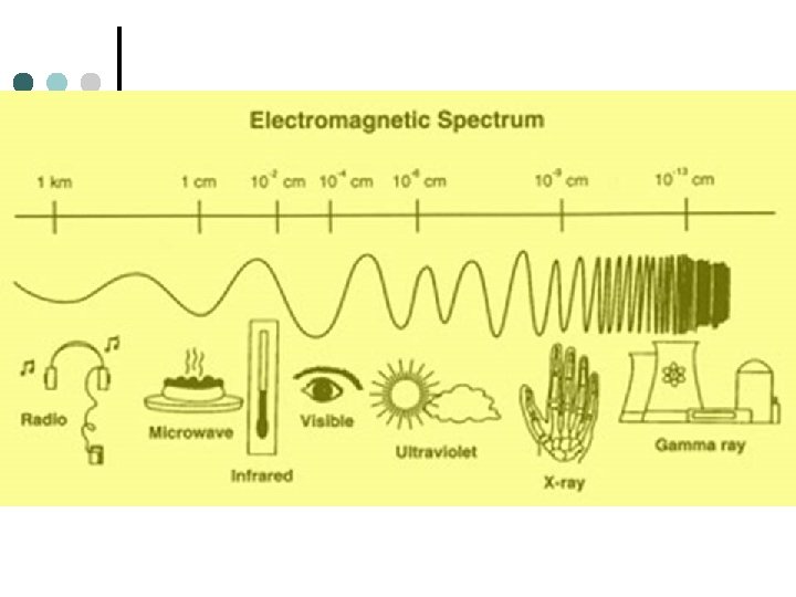
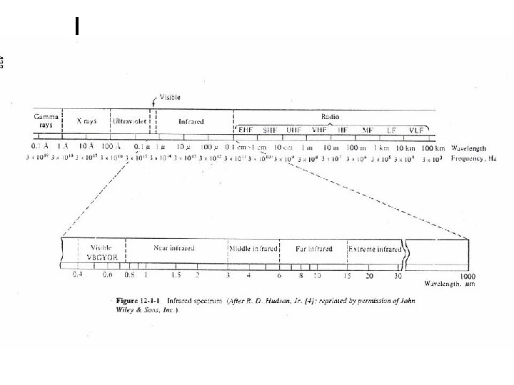
Detalles de las Etapas de Diseño (2) ¢ 2 - Identificar rangos de frecuencia que se pueden usar (Recomendaciones y Normas ITU-R, FCC, IEEE).
The Electromagnetic Spectrum 1 Hz 1 k. Hz 1 MHz 60 Hz ELECTRIC POWER 1 GHz FREQUENCY Hz 1015 Hz 1018 Hz 1012 FM AM RADIO TV 1021 Hz 1024 Hz 1027 Hz VISIBLE LIGHT MICROWAVES RADIO FREQUENCY RADIATION INFRARED ULTRAVIOLET X-RAYS NON-IONIZING RADIATION 3 x 10⁸ 4. 1 x 10 -15 e. V 3 x 10⁵ 3 x 10² 3 x 10 -1 3 x 10 -4 3 x 10 -7 3 x 10 -10 WAVELENGTH (METERS) 4. 1 x 10 -6 4. 1 x 100 e. V ENERGY (ELECTRON VOLTS) GAMMA COSMIC IONIZING RADIATION 3 x 10 -13 3 x 10 -16 3 x 10 -19 4. 1 x 10¹² e. V
Hay que tener en cuenta las normas que rigen las telecomunicaciones A nivel mundial, las regulaciones las hace la Unión Internacional de Telecomunicaciones http: //www. itu. int/home/ y la IEEE recomienda http: //www. ieee 802. org/11/. Pero en todos los países hay agencias que regulan a nivel nacional. Por ejemplo, en USA es la FCC http: //www. fcc. gov/. Asignación: Visitar los sitios y aprender qué hace cada agencia. Tener en cuenta que algunas regulaciones de FCC, por ejemplo, están siendo cuestionadas. Las normas pueden variar ligeramente de un país a otro.
Ver en sitio de Web. Ct FCC Part_15_2_1_06. pdf, Part_15_Survey. ppt Will Changes to Part 15 of the FCC Rules & Regulations Encourage Innovation? Opinions of Members of the FCC Technological Advisory Council
Un estándar de IEEE que ha revolucionado las telecomunicaciones (ver Web. Ct, documento 802_11 tut. pdf)
Lectura recomendada: Unlicenced Wireless Broadband profiles (by Matt Barranca). Ver documento en Web. Ct, New. American. Unlicensed. pdf
El uso libre de bandas de frecuencia
Detalles de las Etapas de Diseño (3) ¢ 3 - Identificar alternativas de transmisión y mecanismos de propagación.
ACCESS SCHEMES ¢ For radio systems there are two resources, frequency and time. Division by frequency, so that each pair of communicators is allocated part of the spectrum for all of the time, results in Frequency Division Multiple Access (FDMA). Division by time, so that each pair of communicators is allocated all (or at least a large part) of the spectrum for part of the time results in Time Division Multiple Access (TDMA). In Code Division Multiple Access (CDMA), every communicator will be allocated the entire spectrum all of the time. CDMA uses codes to identify connections. http: //www. umtsworld. com/technology/cdmabasics. htm
ACCESS SCHEMES http: //www. umtsworld. com/technology/cdmabasics. htm
CODING ¢ CDMA uses unique spreading codes to spread the baseband data before transmission. The signal is transmitted in a channel, which is below noise level. The receiver then uses a correlator to despread the wanted signal, which is passed through a narrow bandpass filter. Unwanted signals will not be despread and will not pass through the filter. Codes take the form of a carefully designed one/zero sequence produced at a much higher rate than that of the baseband data. The rate of a spreading code is referred to as chip rate rather than bit rate. See coding process page for more details. http: //www. umtsworld. com/technology/cdmabasics. htm
CODING
POWER CONTROL ¢ CDMA is interference limited multiple access system. Because all users transmit on the same frequency, internal interference generated by the system is the most significant factor in determining system capacity and call quality. The transmit power for each user must be reduced to limit interference, however, the power should be enough to maintain the required Eb/No (signal to noise ratio) for a satisfactory call quality. Maximum capacity is achieved when Eb/No of every user is at the minimum level needed for the acceptable channel performance. As the MS moves around, the RF environment continuously changes due to fast and slow fading, external interference, shadowing , and other factors. The aim of the dynamic power control is to limit transmitted power on both the links while maintaining link quality under all conditions. Additional advantages are longer mobile battery life and longer life span of BTS power amplifiers See UMTS power control page for more details. http: //www. umtsworld. com/technology/cdmabasics. htm
MULTIPATH AND RAKE RECEIVERS ¢ One of the main advantages of CDMA systems is the capability of using signals that arrive in the receivers with different time delays. This phenomenon is called multipath. FDMA and TDMA, which are narrow band systems, cannot discriminate between the multipath arrivals, and resort to equalization to mitigate the negative effects of multipath. Due to its wide bandwidth and rake receivers, CDMA uses the multipath signals and combines them to make an even stronger signal at the receivers. CDMA subscriber units use rake receivers. This is essentially a set of several receivers. One of the receivers (fingers) constantly searches for different multipaths and feeds the information to the other three fingers. Each finger then demodulates the signal corresponding to a strong multipath. The results are then combined together to make the signal stronger. http: //www. umtsworld. com/technology/cdmabasics. htm
Rangos de f (ELF, ULF, VLF, MF, HF, VHF, UHF, EHF…) y diferentes mecanismos de propagación. LOS ¢ Surface wave ¢ Sky wave ¢ Troposcatter ¢ etc ¢
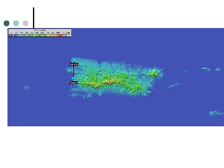
Detalles de las Etapas de Diseño (4) ¢ 4 - Analizar preliminarmente las posibles rutas de propagación (usar Google Earth, USGS).
Ver Web. Ct, Google Earth
UPRM-UPRAguadilla Geography U. S. Department of the Interior, U. S. Geological Survey, National Center, EROS || Not accurate for measurement purposes. || Visit us at http: //gisdata. usgs. net See Tutorial in http: //seamless. usg. gov/Website/seamless/ viewer. php)
Western PR
Zoom to Area XY Enter coordinates of points
Measure distance between points Measure heights, do profile
Tener en cuenta que… ¢ ¢ ¢ En los plots de USGS las distancias están en millas, y las alturas en metros o en píes. Tener en cuenta las distancias entre los puntos (Ex. UPR Aguadilla-UPRM es de 17. 34 millas, o 27. 9 km). Hay que medir individualmente las alturas de los puntos extremos (Ex. note que UPR Aguadilla está a 47 m sobre el nivel del mar, HASL=47 m). UPRM está a 119. 337 m HASL. Estos datos servirán para constatar las alturas de los puntos extremos. Hay que ser cuidadosos al colocar los extremos del plot en el mapa de USGS. Note que las antenas estarán a cierta altura sobre el nivel de tierra (HAGL).
5 points plot…muy pocos datos
10 points plot…todavía muy pocos
20 points plot…tampoco, necesitamos al menos 100
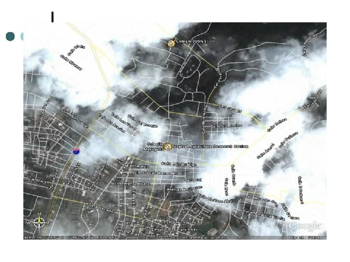
Detalles de las Etapas de Diseño (5) ¢ 5 - Identificar las características principales de las rutas de propagación (podrían usarse mapas de escala 1: 25, 000 de USGS en el web).
Point 1: UPR-Aguadilla (18. 46 N, - 67. 11 W) Point 2: UPR-Mayagüez (18. 21 N, -67. 13 W) Distance: 17. 34 miles(27. 90 km) (50 points, using http: //seamless. usg. gov/Website/seamless/viewer. php)
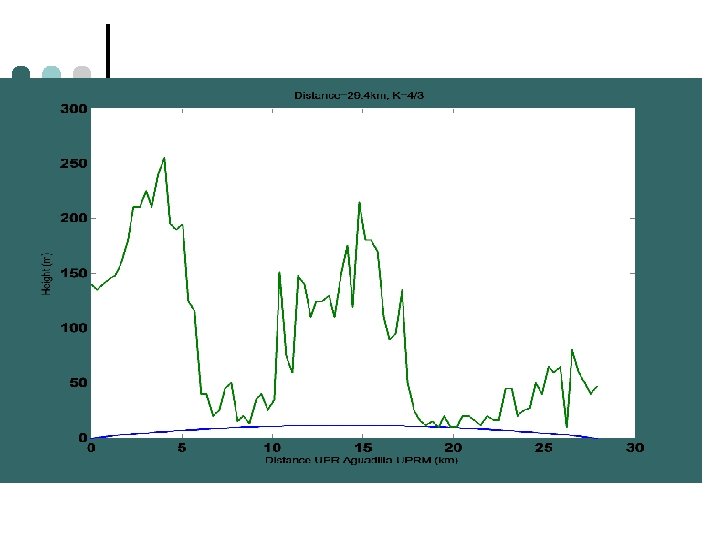
Detalles de las Etapas de Diseño (6) ¢ 6 - Seleccionar una ruta y obtener la base de datos topográficos (Digital Elevation Models, USGS).
Point 1: UPR-Aguadilla (18. 46 N, - 67. 11 W) Point 2: UPR-Mayagüez (18. 21 N, -67. 13 W) Distance: 17. 34 miles(27. 90 km) ( 100 points, using http: //seamless. usg. gov/Website/seamless/viewer. php)
Point 1: UPR-Aguadilla (18. 46 N, - 67. 11 W) Point 2: UPR-Mayagüez (18. 21 N, -67. 13 W) Distance: 17. 34 miles(27. 90 km) (100 points, using http: //seamless. usg. gov/Website/seamless/viewer. php)
Ejemplo de pequeño programita en Matlab para hacer un patrón de perfiles topográficos (demostrar cada término) >> S=27. 90; ¢ >> b=0. 0589 ¢ >> D 1=0: 27. 9/99: 27. 9; ¢ >> h 1=b*(S-D 1). *D 1; ¢ >> y=[140 135 140 145 148 160 180 210…vector of 100 elements]; ¢ >> plot(D 1, h 1, D 1, y) ¢
m-file for plotting function testing 1 b=0. 0589; S=50; D 1=0: 0. 001: 50; h 1=b*(S-D 1). *D 1; plot (D 1, h 1) hold plot (D 1, h 1+50) hold on plot (D 1, h 1+100) hold on plot (D 1, h 1+150) hold on plot (D 1, h 1+200) hold on plot (D 1, h 1+250) hold on
!Ojo! Plot correcto, pero líneas horizontales incorrectas. Pasan cosas así cuando no se sabe en qué se basa el código.
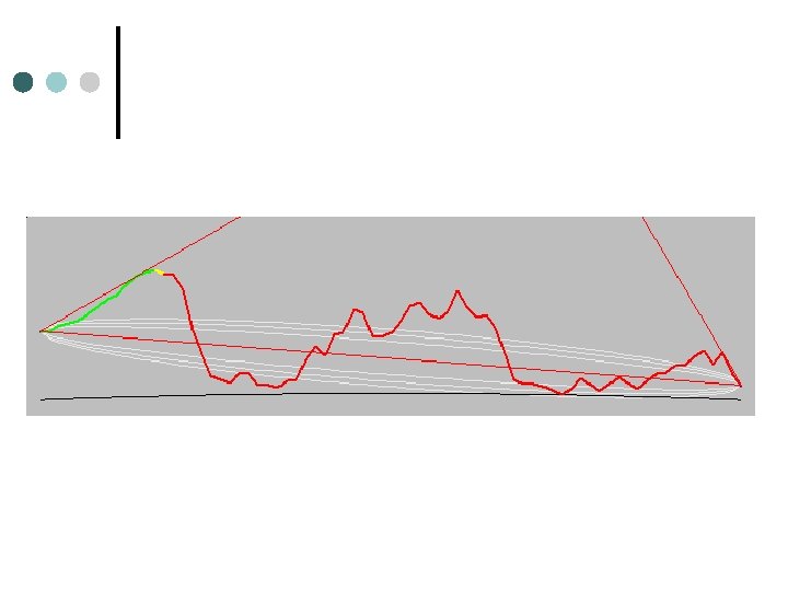
Detalles de las Etapas de Diseño (7) ¢ 7 - Usar un software package (Radio Mobile, Radiosoft Comstudy, Planner, etc. ) para analizar rutas y escoger alturas de antenas según requisitos de Zonas de Fresnel, reflexiones, etc.
Software comercial para diseñar radio-enlaces (si se usa algo así, hay que entender de dónde viene cada cosa) http: //beradio. com/products/radio_radiosoft_comstudy/
Ver en Web. Ct Radio. Mobil. doc (direcciones para ver instrucciones sobre uso e instalación)
Coordenadas, Altura Aguadilla 18. 4606 N -67. 11101 W 133. 353 m Mayaguez 18. 21053 N -67. 13 W ¢ ¢ 39. 081 m
Point 1: UPR-Aguadilla (18. 46 N, - 67. 11 W) Point 2: UPR-Mayagüez (18. 21 N, -67. 13 W) Distance: 17. 34 miles(27. 90 km) (100 points, using http: //seamless. usg. gov/Website/seamless/viewer. php)
Compare…calidades de las diferentes bases de datos
Atmospheric Effects ¢ ¢ If the radio beam propagates in free space with NO ATMOSPHERE, the path is a straight line. Through the earth’s atmosphere, variations in εr along the path causes the ray path to become curve. Atmospheric gases absorb and scatter the radio path energy. n = (εr )1/2 variations affect the curvature of the ray path.
Taken from R. Freeman, Radio System for Telecommunications, Wiley 2002
Taken from R. Freeman, Radio System for Telecommunications, Wiley 2002
Fresnel zone problem (Taken from R. Freeman, Radio System for Telecommunications, Wiley 2002)
Taken from R. Freeman, Radio System for Telecommunications, Wiley 2002
Ground Reflection ¢ ¢ Radio waves reflected from the earth’s surface are generally changed in phase depending on the polarization and the angle of incidence. Horizontally polarized waves are shifted ≈180 o (path length changes ≈ λ/2). The resulting reflections may arrive out of phase with the direct wave. For vertical pol. phase, shift varies between 0 - 180 o, depending on the reflection coeff. Tower heights can be adjusted to move the reflection to a convenient point.
Fading ¢ ¢ ¢ Defined as any time varying of phase, polarization, and/or RSL. The definitions are in terms of refraction, reflection, diffraction, scattering, attenuation, and guiding (ducting) of the radio wave. The terms determine the statistical behavior of fields level, phase, polarization, frequency and spatial selectivity of the fading. Fading is caused by certain terrain geometry and meteorological conditions. All communication systems in the 1 -100 GHz range can suffer fading, including satellite earth terminals operating at low elevation angles and/or in heavy precipitation.
Multipath Fading ¢ ¢ Is the most common type of fading encountered on LOS radiolinks. Could be particularly troublesome on high-bit-rate LOS links. As n = (εr )1/2 changes, multipath fading results owing to the interference between direct rays and ground-reflected wave, or reflections from atmospheric sheets, or other reflections. The fading rate (number of fades/time), and the fading depth (variation of RSL from its free space value in db) are important factors for design engineers. Fade can exceed 20 db on longer LOS paths.
Power Fading Results from a shift of the beam from the receiving antenna due to one or several of the following: -intrusion of earth’s surface or atmospheric layers into the path. -antenna decoupling due to K-factor variations. -partial reflections from elevated layers. -one of the antennas in a ducting formation. -rain in the propagation path. ¢
Fading due to Earth bulge ¢ ¢ ¢ If K < 1 (sub-refractive), power fading depths of 20 -30 db for several hours or more may be expected owing to the diffraction by the earth’s surface. This type of fading may not be normally mitigated by freq. diversity. It may be reduced or completely avoided by the proper adjustment of antenna tower heights. Clearances greater than one Fresnel zone may be required (one Fresnel zone in mountainous regions)!
Some other factors of fading K-Factor Fading ¢ Surface Duct Fading on Over-Water Paths ¢ Duct and layer fading ¢ Taken from R. Freeman, Radio System for Telecommunications, Wiley 2002
Taken from www. umtsworld. com/technology/cdmabasi cs. htm
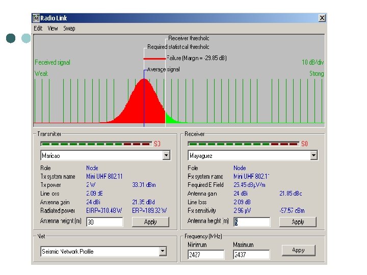
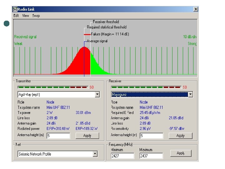
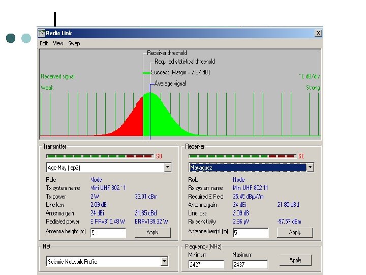
Detalles de las Etapas de Diseño (8) ¢ 8 - Repetir el paso anterior con diferentes condiciones atmosféricas (K = 5/3, 4/3, 1, 2/3). Escoger la ruta y seleccionar preliminarmente el sistema (Tx, Rx, antenas, líneas, etc. ). El paso anterior es ¢ 7 - Usar un software package (Radio Mobile, Radiosoft Comstudy, Planner, etc. ) para analizar rutas y escoger alturas de antenas según requisitos de Zonas de Fresnel, reflexiones, etc.
Una fórmula para ser demostrada y discutida en detalle (path calculations) Pt db = - 171. 5 + 20. log f. MHz + 20. log rkm + 10. log RHz + (Eb/N 0)db + NFdb + - GT db - GR db + LT db + LR db + Aa db
Tener cuidado con el uso de calculadoras…Si no se entienden las fórmulas, puede haber sorpresas
Distance Aguadilla- Mayaguez is 27. 9 km (17. 3 miles) True North Azimuth = 184. 1°, Magnetic North Azimuth = 196. 2°, Elevation angle = -0. 4015° Terrain elevation variation is 222. 5 m
Distance Mayaguez-Aguadilla is 27. 9 km (17. 3 miles) True North Azimuth = 4. 1°, Magnetic North Azimuth = 16. 2°, Elevation angle = 0. 1507° Terrain elevation variation is 222. 5 m
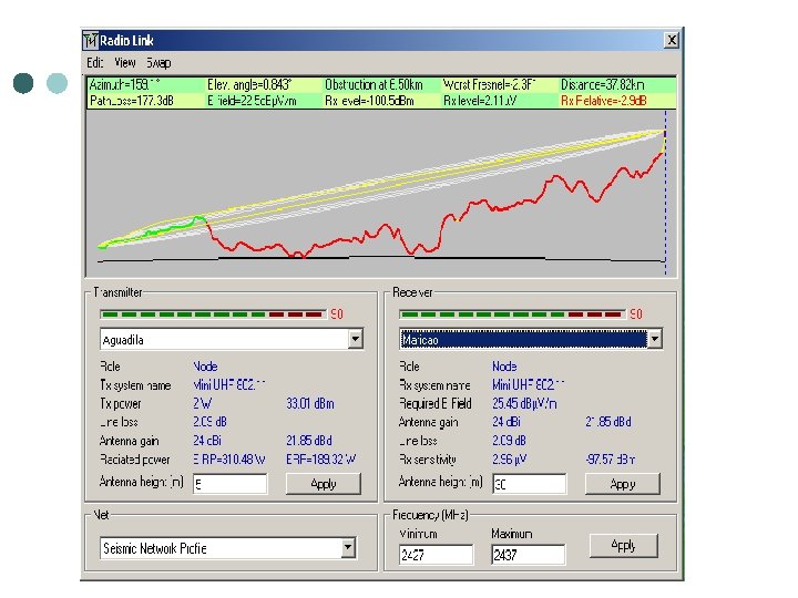
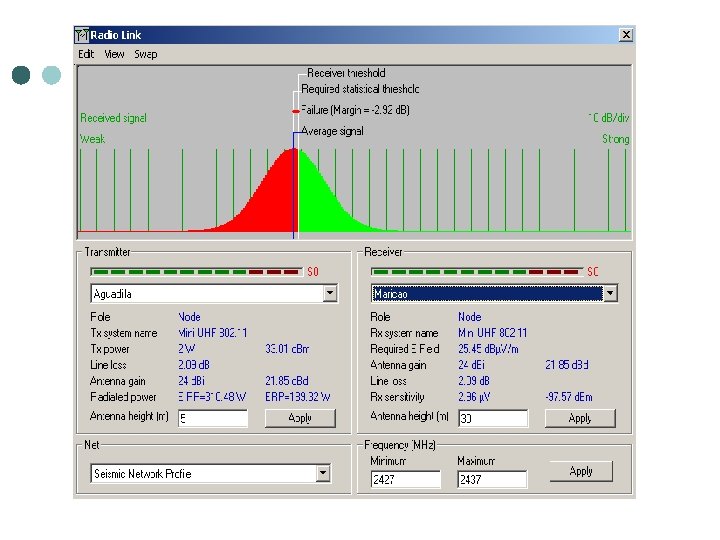
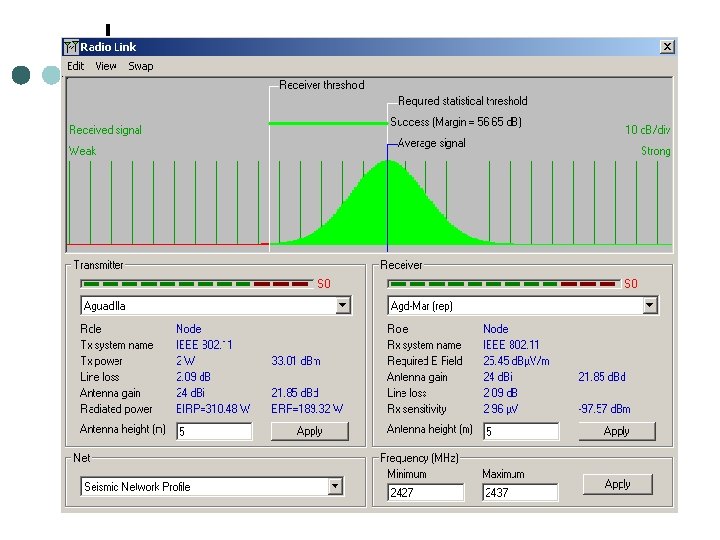
Transmitter (Aguadilla): Tx Power=10 w (40 d. Bm), Gt=5 d. Bi (2. 85 d. Bd), Lt=1 d. B EIRP= 25. 12 W, ERP= 15. 32 W, ht=240 m 2400 MHz ≤ f ≤ 2406 MHz Receiver (Mayagüez): Required E field = 31. 33 d. Bµ/m, Gr=5 d. Bi (2. 85 d. Bd), Lr=1 d. B Rx sensitivity = 0. 75µV ( -109. 5 d. Bm), hr=200 m Azimuth= 184. 10, Elev. angle=-0. 4010 , Clearance at 16. 57 km, Worst Fresnel=3. 01 F 1, r=27. 86 km Path. Loss=127. 3 d. B, E=61. 5 d. BµV/m (at Rx antenna), Rx level=-79. 3 d. Bm Rx level=24. 15µV, Rx relative = 30. 2 d. B !Note que las alturas de las torres son absurdas!
Distance between Aguadilla and Mayaguez is 27. 9 km (17. 3 miles) ¢ ¢ ¢ ¢ ¢ True North Azimuth = 184. 1°, Magnetic North Azimuth = 196. 2°, Elevation angle = -0. 4015° Terrain elevation variation is 222. 5 m Propagation mode is line-of-sight, minimum clearance 3. 0 F 1 at 16. 6 km Average frequency is 2403. 000 MHz Free Space = 128. 9 d. B, Obstruction = -2. 8 d. B, Urban = 0. 0 d. B, Forest = 0. 0 d. B, Statistics = 1. 2 d. B Total propagation loss is 127. 3 d. B System gain from Aguadilla to Mayaguez is 157. 5 d. B System gain from Mayaguez to Aguadilla is 157. 5 d. B Worst reception is 30. 2 d. B over the required signal to meet 50. 000% of time, 50. 000% of locations, and 50. 000% of situations
Detalles de las Etapas de Diseño (9) ¢ 9 - Hacer pruebas de propagación (si hay los medios para tomar muestras), o usar Matlab para simular una señal recibida con los parámetros escogidos preliminarmente en el paso anterior.
Muestra tomada…o simulada, si no hay manera de hacer pruebas de propagación
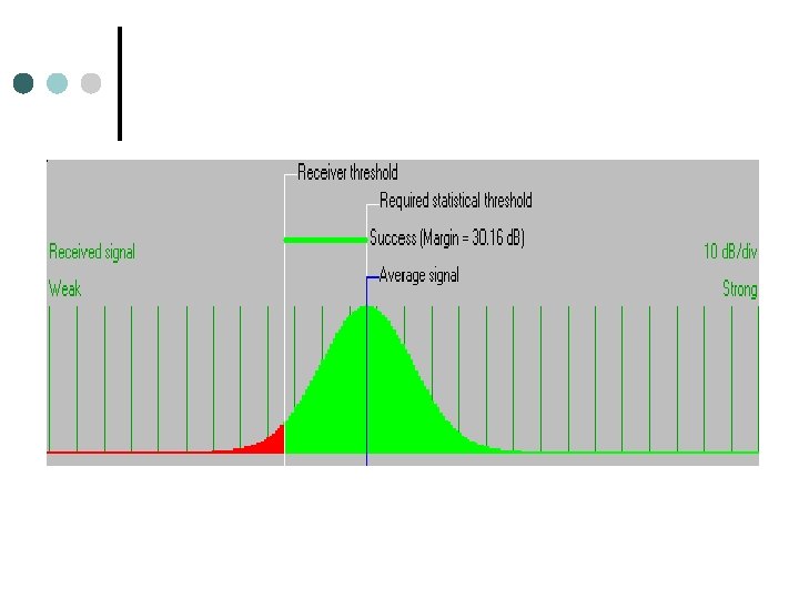
Detalles de las Etapas de Diseño (10) ¢ 10 - Usar Gaussian distribution, y determinar mean, std, etc. de la señal simulada (o muestra recibida) para adecuar el sistema a la confiabilidad de operación especificada.
Detalles de las Etapas de Diseño (11) ¢ 11 - Usar Matlab para comparar algunos resultados, haciendo el perfil con la base de datos topográficos y observando niveles de señal (reales o simulados), de acuerdo al paso anterior.
¢ Radio Mobile for Windows Version 7. 1 Name Aguadilla Antenna height 240(m) Name Mayaguez Antenna height 200(m) Frequency 2. 403(GHz) Earth curvature factor K = 1. 33331675899808 ¢ Distance(km) Elevation(m) Path. Loss(d. B) ¢ ¢ ¢ ¢ ¢ ¢ ¢ ¢ ¢ ¢ ¢ 0000. 377 0000. 753 0001. 130 0001. 506 0001. 883 0002. 259 0002. 636 0003. 012 0003. 389 0003. 765 0004. 142 0004. 518 0004. 895 0005. 271 0005. 648 0006. 024 0006. 401 0006. 777 0007. 154 0007. 530 0007. 907 0008. 283 0008. 660 0009. 036 0009. 413 0009. 789 0010. 166 0010. 542 0010. 919 0011. 295 0011. 672 0012. 048 0012. 425 0012. 801 0013. 178 0013. 554 0013. 931 0014. 307 0014. 684 0015. 060 0133. 4 0135. 0 0143. 7 0148. 7 0152. 6 0163. 1 0174. 3 0187. 8 0194. 8 0211. 8 0226. 1 0232. 5 0237. 4 0231. 3 0227. 6 0200. 8 0129. 8 0087. 6 0048. 2 0041. 7 0036. 2 0053. 1 0050. 8 0031. 0 0029. 8 0027. 1 0037. 5 0038. 2 0073. 7 0098. 7 0082. 8 0118. 4 0122. 5 0163. 6 0156. 8 0116. 4 0114. 9 0122. 2 0141. 7 0169. 2 0174. 6 0 0 0 0 0 0 0 0 0 0 0 0 0 0 0 0 0 0 0 0 000. 0 095. 3 104. 2 102. 7 109. 9 106. 6 109. 4 108. 1 109. 2 110. 1 111. 3 112. 0 115. 4 113. 6 119. 2 114. 2 118. 8 117. 4 115. 8 119. 9 120. 0 121. 1 117. 4 118. 7 119. 1 123. 9 121. 9 120. 0 121. 0 120. 8 121. 0 121. 8 125. 8 122. 5 122. 4 122. 2
Observe como fluctúa la atenuación (cerca de r=0 hay indeterminación)
Detalles de las Etapas de Diseño (11) ¢ ¢ 12 - Dimensionar de nuevo el sistema, con base en los resultados de los dos pasos anteriores. !Tener en cuenta cálculos de SAR, aunque se use baja potencia!
International Commission on Non-Ionizing Radiation Protection (ICNIRP) Guidelines for human exposure limits. Human Exposure to Electromagnetic Fields Fundamental information regarding human interaction with electromagnetic radiation, covering several aspects of incident and internal field dosimetry, thermal body response, biological effects, measurement techniques and safety standards regarding the possible radiation hazard with reference to the existing limits.
Conviene saber la diferencia entre Ionizing vs. Non-Ionizing Radiation, aunque las ondas EM usadas aquí no son de frecuencias ionizantes ¢ ENERGY= f * h Where h=Plancks constant = 6. 63 x 10 -34 joule seconds f = frequency l The higher the frequency, the higher the energy l
Ionizing vs. Non-Ionizing Radiation At a frequency of approx. 2. 420 x 106 GHz the energy level is sufficient to ionize water molecules. ¢ Therefore, frequencies at or above this level are classified as “Ionizing” ¢
Efectos de la Radiación Ionizante Un rayo X de 3 x 10¹⁸ Hz tiene fotones con energía de hf=(6. 626 x 10 -34). (3 x 10¹⁸)=1. 878 x 10 -16 Jouls, que equivale a 12. 4 Ke. V. ¢ En el rango UV, una onda de 2. 42 x 1015 Hz tiene fotones de 10 e. V. Para ionizar un átomo se requiere que el fotón que choca con el electrón tenga energía por lo menos igual a la que lo mantiene ligado al núcleo. ¢
Efectos de la rad. Ioniz. (cont. ) Material Energía Ionizante Hidrógeno 13. 6 e. V Sodio gaseoso 5. 1 e. V Agua 12. 4 e. V son suficientes para ionizar una molécula de agua. Una onda de f>1015 Hz es radiación ionizante. La energía de un fotón en particular es muy pequeña, pero el número de fotones en un haz de moderada intensidad es enorme. La ionización produce profundos cambios químicos que pueden ser irreversibles.
Energía de los fotones de algunos servicios de RF TV de UHF de 700 MHz 2. 88 x 10 -6 e. V ¢ Radar de microondas de 10 GHz 4. 12 x 10 -5 e. V ¢ Onda milimétrica de 300 GHz 1. 24 x 10 -3 e. V ¢ Luz visible de 6 x 10⁵ GHz 2. 47 e. V Comparar con Radiación UV de 10 x 107 GHz 41. 2 e. V Rayos X blandos de 109 GHz 4120. 0 e. V Rayos X duros de 1012 GHz 4. 120 x 105 e. V ¢
Pero la radiación no-ionizante también puede ser muy peligrosa Las ondas de RF pueden producir vibraciones y oscilaciones rotacionales en las moléculas, que se traducen en calentamiento y otros efectos. ¢ Esto puede dar lugar a cambios drásticos en las substancias orgánicas e inorgánicas. ¢
CW or Average Power (W) Maximum Limits of Average Power from Man-made sources 106 Gridded Tube 104 Avalanche diode 102 Solid State 1 Frequency Cyclotron Tubes Microwave Tubes 0. 01 0. 1 1 10 1000 GHz
Power Output Levels UHF Transmitter (120 k. W) AM/FM Transmitter 5 -50 k. W) Microwave Oven (800 W) Mobile Radio (50 W) C. B. Radio (5 W) Microwave Radiation by Humans (3. 5 W) Cellular Phone (0. 6 W) Childrens Walkie-Talkie (0. 15 W) Police Radar (0. 015 W) Door Opener (0. 005 W) Firefly (0. 0005 W)
RF Energy and the Human Body ¢ There are many factors that affect absorption into the human body Dielectric Composition l Size of the Body l Shape, Orientation and Polarization l Complexity of the RF field l
1. Dielectric Composition (ver, por ejemplo, Ishimaru, EM Wave Propagation, Prentice Hall, 2002) ¢ Since the human body has a different dielectric constant (Є) than free space, field measurements are performed where the front surface of the body would be. RF energy typically passes through the fatty tissue and is deposited in the muscle or brain tissues.
Muscle 7 70 60 50 40 30 6 5 4 3 20 2 1 0. 1 Fat Penetration Depth vs. Frequency vs. Different tissues (cm’s) 10 0. 3 1. 0 3. 0 10 GHz
Penetration depth vs. Frequency Penetration Depth in cm. 1000 10 l in cm. l / 100 10 l / 30 1. 0 10 l / 10 1000 10, 000 MHz
2. Size of the Body ¢ There are different absorption characteristics based on the size of the body and the wavelength • A. l > The body In this region, there is little absorption and a uniform or equal distribution of energy. The impedance of the body increases as the wavelength increased. Safety standards are based on shock or burn hazards rather than direct absorption.
2. Size of the Body (Cont’d) • l ~ = The Body In this region, the absorption is highest and the energy is distributed unequally. Hot spots may be generated. • l < The Body Lower absorption of energy and heating confined to irradiated area.
RF Absorption vs. Frequency 1. 0 SAR Induced in a 1. 75 m high Human Exposed to 1 m. W/cm 2 RF Field Specific Absorption Rate (W/kg) E - Polarization 0. 1 H - Polarization . 01 K - Polarization E Antenna . 001 K . 0001 10 Frequency H 30 100 (MHz) Radiation 300 1 3 10 (GHz) 30 100
RF Absorption vs. Frequency 1. 0 Upper Limit SAR for the range of human beings from infant to adult Average SAR (W/kg) 0. 3 0. 1 0. 03 0. 01 0. 003 0. 001 10 Numerical Calculations based on a block model of man in conductive contact with ground One year old child in conductive contact with ground 30 Prolate model of a human infant 60 100 Frequency (MHz) 300 600 1000
3. Shape, Orientation and Polarization ¢ The Human body in a vertical position absorbs 10 times more energy in a vertically vs. horizontally polarized emission. l RF energy can be focused in common, workplace environments. Reflective environments (screen rooms, sides of buildings, etc. ) can enhance the fields in certain conditions.
4. Complexity of the Fields Most all standards are based on the far field relationships and their interaction with the body. l Near field exposures are difficult to measure and almost impossible to calculate. l Combined with the three previous factors determining absorption, the total variables become staggering. l
Non-thermal Effects Many have been postulated, but none have been proven ¢ Melatonin suppression is an effect that is not completely understood. ¢ GSM phones under evaluation because of modulation phenomena. ¢
Cellular Phone Studies ¢ RF Exposure in the vicinity of portable communication devices Usually antennas have cylindrical symmetry l Power density is not a meaningful parameter l The exposed body may cause a substantial alteration of the RF source characteristics l The exposed body and the antenna become practically one source of RF fields l
Detalles de las Etapas de Diseño (12) ¢ 12 - Identificar proveedores de los equipos y componentes apropiados y hacer selección final del sistema, ajustado a los requisitos del diseño y a las recomendaciones y normas de ITU-R, FCC, IEEE. Ejemplo de proveedor: www. freewave. com/
N-Male Connector, 0. 25 d. B loss Cisco Aironet 350 Wireless Bridge Laptop (Linux) Proxim Orinoco Wireless PC Card Hyperlink 2. 4 GHz, 24 d. Bi Antenna Times Microwave Systems LMR-400 Coax Cable TTX 13 / VTX 13 Transmitter TRX 23/VRX 23 Receiver
Receptor TRX Series L-3 Telemetry West Receptor
Transmisor TTX 13 Series L-3 Telemetry West
Detalles de las Etapas de Diseño (13) Elaborar documentos: Lista de equipos, antenas, cables, torres, …y componentes necesarios para instalar el sistema. ¢ Especificar mediciones requeridas para optimizar el sistema y mantener operativo su funcionamiento. ¢
Spectrum Analyzer ¢ Measurements: Noise Floor l Bandwidth l Noise Figure l Peak Power l Gain l 1 d. B Compression Point l
Noise Figure (NF) Noise Figure Measurement Setup: Spectrum Analyzer DUT RF Noise Source Pre Amplifier Power Supply @ 4. 5 V
1 d. B Compression Point ¢ Measure of what is less than expected by 1 d. B (saturation) ¢ Determine the utility of an amplifier ¢ Measure linearity ¢ Determine Dynamic Range (region of operation)
1 d. B Compression Point Setup: Spectrum Analyzer RF Signal Generator DUT Pre Amplifier Power Supply @ 4. 5 V
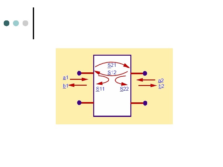
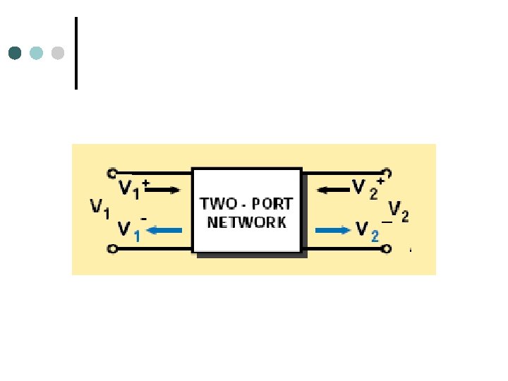
Network Analyzer S Parameters of an RF/Microwave Device ¢ Transmission (S 12, S 21) Reflection (S 11, S 22) Impedance (Matching) VSWR Verify Bandwidth ¢Resonant Frequencies ¢
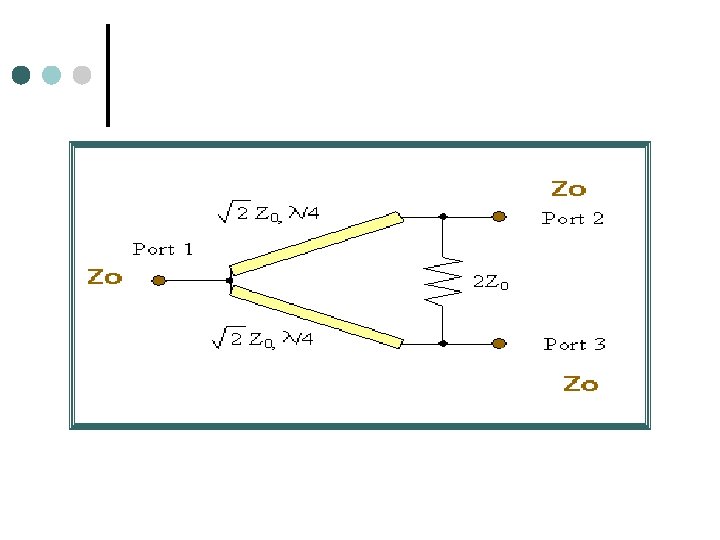
Wilkinson Power Divider
Detalles de las Etapas de Diseño ¢ 13 - Identificar proveedores de los equipos y componentes apropiados y hacer selección final del sistema, ajustado a los requisitos del diseño y a las Recomendaciones y Normas de ITUR, FCC, IEEE, OSHA. ¢ 14 - Hacer lista de equipos, antenas, torres, cables…y componentes necesarios para instalar el sistema. ¢ 15 - Elaborar documento explicativo sobre las mediciones necesarias para optimizar el funcionamiento del sistema. ¢ 16 - Hacer un Resumen Ejecutivo.
!Si…este es el último slide! Gracias por su atención a esta parte del curso