Radar Systems Analysis and Design Using MATLAB Chap

Radar Systems Analysis and Design Using MATLAB Chap. 6 Matched Filter and the Radar Ambiguity Function 6. 4 ~

6. 4 The Radar Ambiguity Function 1 � The radar ambiguity function (|χ|2) represents the output of the matched filter, and it describes the interference caused by range and/or Doppler of a target when compared to a reference of equal RCS. � χ(τ; fd)=χ(0; 0) is equal to the matched filter output that is matched perfectly to the signal reflected from the target of interest. (=returns from the nominal target are located at the origin of the ambiguity function. ) � χ(τ; fd)=χ(nonzero; nonzero) represents returns from some range and Doppler different from those for the nominal target.

6. 4 The Radar Ambiguity Function (cont’d) 2 � Matched filter response: χ(τ; fd) - obtained by correlating a signal with its doppler-shifted and timetranslated version. uncertainty function: |χ(τ; fd)| ambiguity function: |χ(τ; fd)|2

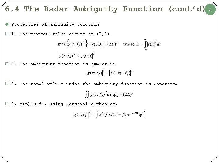
6. 4 The Radar Ambiguity Function (cont’d) 3 u Properties of Ambiguity function � 1. The maximum value occurs at (0; 0). � 2. The ambiguity function is symmetric. � 3. The total volume under the ambiguity function is constant. � 4. s(t)↔S(f), using Parseval’s theorem,

6. 5 Examples of the Ambiguity Function 4 � The ideal radar ambiguity function is represented by a spike of infinitesimal width that peaks at the origin and is zero everywhere else. u 6. 5. 1 Single Pulse Ambiguity Function � Normalized rectangular pulse s(t)

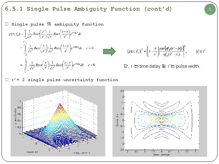
6. 5. 1 Single Pulse Ambiguity Function (cont’d) � Single pulse 의 ambiguity function 단, τ 는 time delay 및 τ’는 pulse width. � τ’= 2 single pulse uncertainty function 5

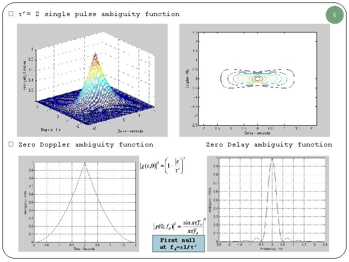
� τ’= 2 single pulse ambiguity function � Zero Doppler ambiguity function 6 Zero Delay ambiguity function First null at fd=± 1/τ’

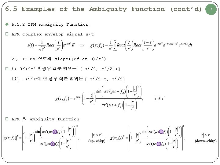
6. 5 Examples of the Ambiguity Function (cont’d) u 6. 5. 2 LFM Ambiguity Function � LFM complex envelop signal s(t) 단, μ=LFM 신호의 slope((Δf or B)/τ’) � i) 0≤τ≤τ’인 경우 적분 범위는 [-τ’/2, τ’/2+τ] ii) -τ’≤τ≤ 0 인 경우 적분 범위는 [-τ’/2 -τ, τ’/2] � LFM 의 ambiguity function 7

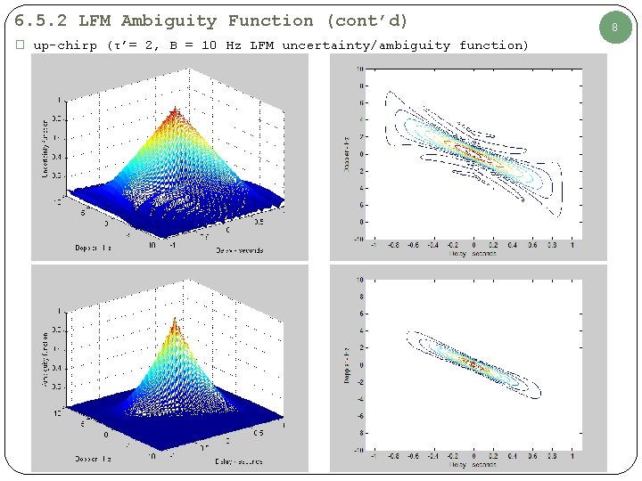
6. 5. 2 LFM Ambiguity Function (cont’d) � up-chirp (τ’= 2, B = 10 Hz LFM uncertainty/ambiguity function) 8

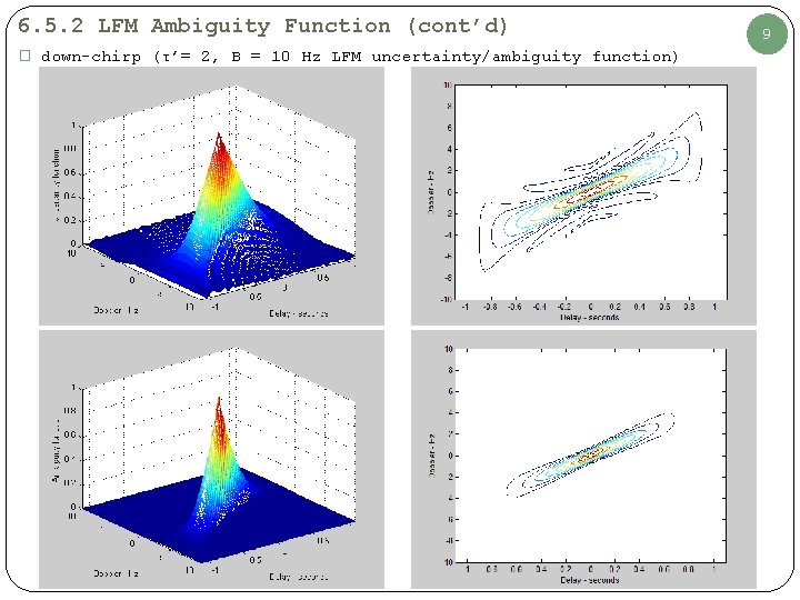
6. 5. 2 LFM Ambiguity Function (cont’d) � down-chirp (τ’= 2, B = 10 Hz LFM uncertainty/ambiguity function) 9

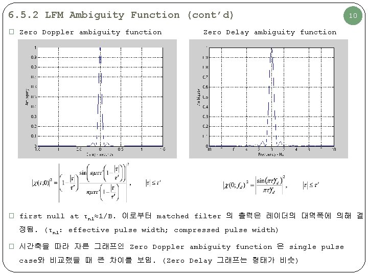
6. 5. 2 LFM Ambiguity Function (cont’d) � Zero Doppler ambiguity function 10 Zero Delay ambiguity function � first null at τn 1≈1/B. 이로부터 matched filter 의 출력은 레이더의 대역폭에 의해 결 정됨. (τn 1: effective pulse width; compressed pulse width) � 시간축을 따라 자른 그래프인 Zero Doppler ambiguity function 은 single pulse case와 비교했을 때 큰 차이를 보임. (Zero Delay 그래프는 형태가 비슷)

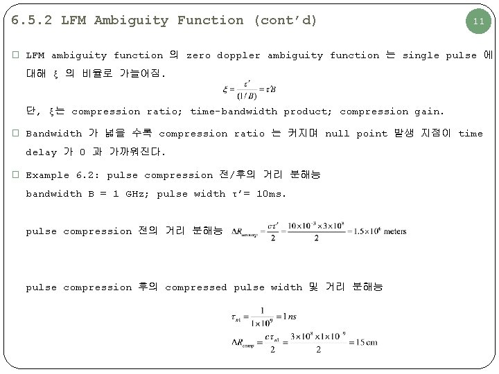
6. 5. 2 LFM Ambiguity Function (cont’d) 11 � LFM ambiguity function 의 zero doppler ambiguity function 는 single pulse 에 대해 ξ 의 비율로 가늘어짐. 단, ξ는 compression ratio; time-bandwidth product; compression gain. � Bandwidth 가 넓을 수록 compression ratio 는 커지며 null point 발생 지점이 time delay 가 0 과 가까워진다. � Example 6. 2: pulse compression 전/후의 거리 분해능 bandwidth B = 1 GHz; pulse width τ’= 10 ms. pulse compression 전의 거리 분해능 pulse compression 후의 compressed pulse width 및 거리 분해능

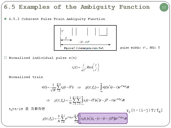
6. 5 Examples of the Ambiguity Function 12 u 6. 5. 3 Coherent Pulse Train Ambiguity Function pulse width: τ’, PRI: T � Normalized individual pulse s(t) Normalized train t 1=t-i. T 로 치환하면 χ1[τ-(i-j)T; fd]

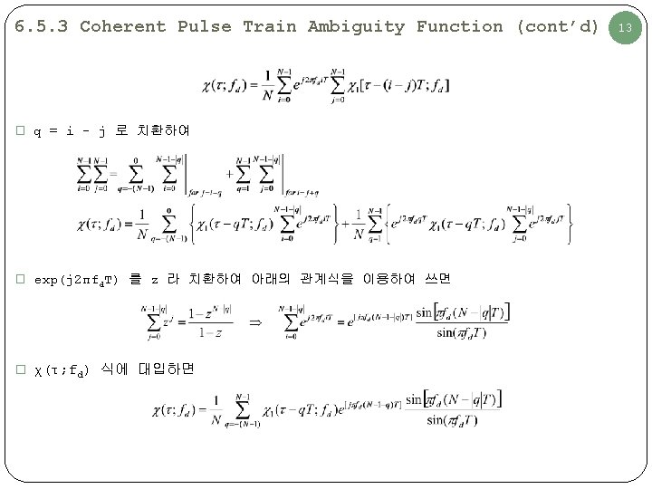
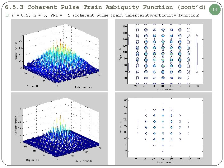
6. 5. 3 Coherent Pulse Train Ambiguity Function (cont’d) � τ’= 0. 2, n = 5, PRI = 1 (coherent pulse train uncertainty/ambiguity function) 14

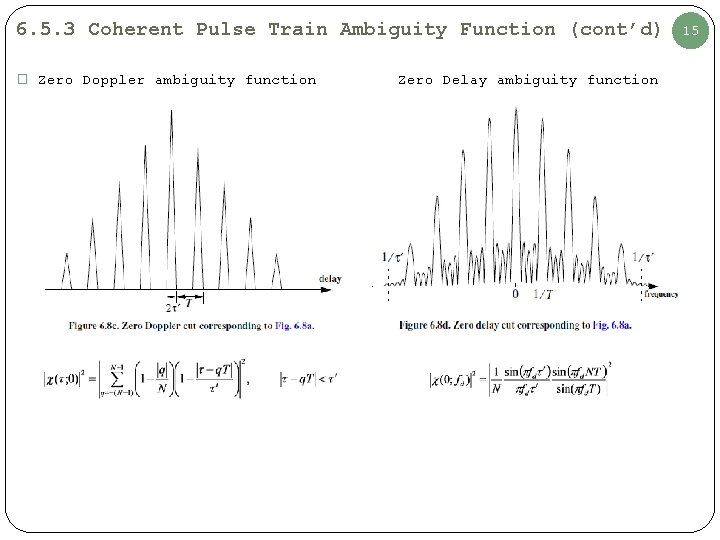
6. 5. 3 Coherent Pulse Train Ambiguity Function (cont’d) � Zero Doppler ambiguity function Zero Delay ambiguity function 15

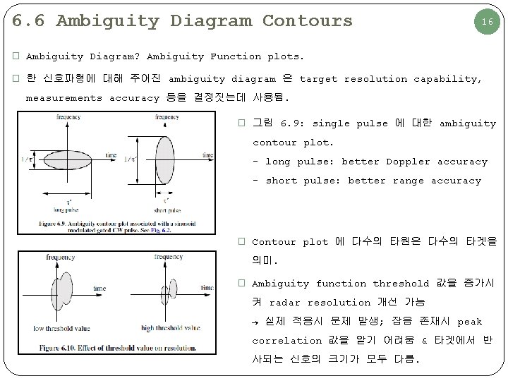
6. 6 Ambiguity Diagram Contours 16 � Ambiguity Diagram? Ambiguity Function plots. � 한 신호파형에 대해 주어진 ambiguity diagram 은 target resolution capability, measurements accuracy 등을 결정짓는데 사용됨. � 그림 6. 9: single pulse 에 대한 ambiguity contour plot. - long pulse: better Doppler accuracy - short pulse: better range accuracy � Contour plot 에 다수의 타원은 다수의 타겟을 의미. � Ambiguity function threshold 값을 증가시 켜 radar resolution 개선 가능 → 실제 적용시 문제 발생; 잡음 존재시 peak correlation 값을 알기 어려움 & 타겟에서 반 사되는 신호의 크기가 모두 다름.

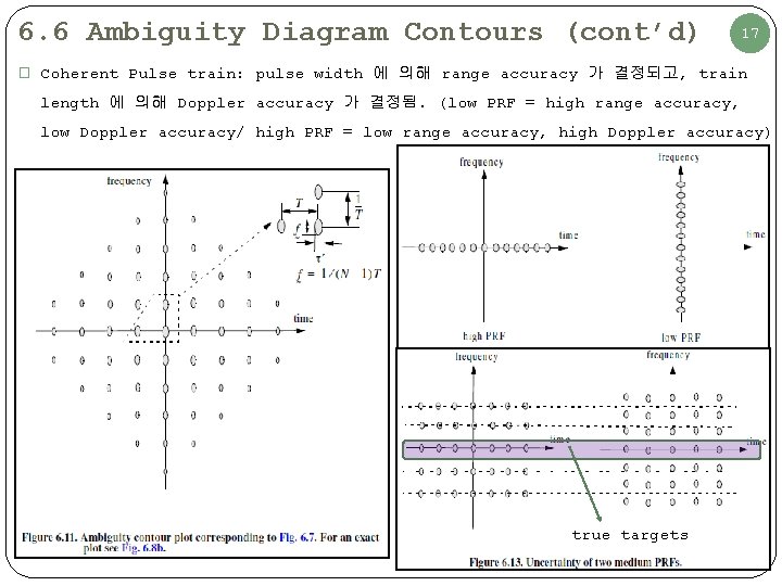
6. 6 Ambiguity Diagram Contours (cont’d) 17 � Coherent Pulse train: pulse width 에 의해 range accuracy 가 결정되고, train length 에 의해 Doppler accuracy 가 결정됨. (low PRF = high range accuracy, low Doppler accuracy/ high PRF = low range accuracy, high Doppler accuracy) true targets

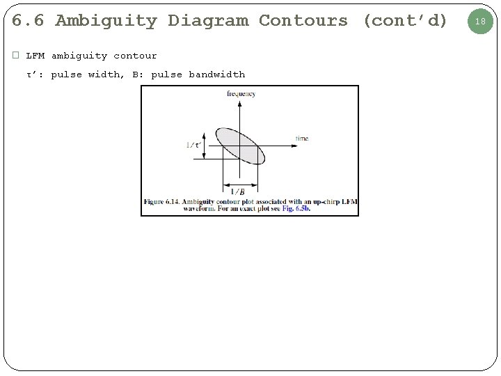
6. 6 Ambiguity Diagram Contours (cont’d) � LFM ambiguity contour τ’: pulse width, B: pulse bandwidth 18

Radar Systems Analysis and Design Using MATLAB Chap. 7 Pulse Compression 7. 1 ~ 7. 2

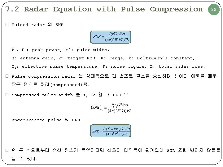
7. 2 Radar Equation with Pulse Compression 22 � Pulsed radar 의 SNR 단, Pt: peak power, τ’: pulse width, G: antenna gain, σ: target RCS, R: range, k: Boltzmann’s constant, Te: effective noise temperature, F: noise figure, L: total radar loss. � Pulse compression radar 는 상대적으로 긴 변조된 펄스를 송신하며 레이더 에코를 매우 짧은 펄스로 처리(compressed)함. � compressed pulse width 를 τc 라 할 때 SNR 은 uncompressed pulse 의 SNR � 위 두 식으로부터 송신 펄스가 동일하다면 신호의 대역폭에 관계없이 SNR 또한 변하지 않음을 알 수 있다.