CONTINUATION OF The molecular rve Hamiltonian and Schroedinger

CONTINUATION OF: The molecular rve Hamiltonian and Schroedinger Eqn. The coordinates and approximations

After XYZ and separating Ttrans To solve this equation we change coordinates and make approximations

XYZ ξηζ and then the Born-Opp Approx We change coordinates by shifting to a (ξηζ) axis system that is oriented as the XYZ, and space-fixed XYZ, axis systems but which has origin at the NUCLEAR centre of mass. In these coordinates we have Hrve = Te + TN + Vee + VNN + VNe The KE is completely separable into electronic and nuclear parts. BUT the V is not separable because of VNe is the “glue” that holds the molecule together so we cannot neglect it.

XYZ ξηζ and then the Born-Opp Approx We change coordinates by shifting to a (ξηζ) axis system that is oriented as the XYZ, and space-fixed XYZ, axis systems but which has origin at the NUCLEAR centre of mass. In these coordinates we have (see p 185 in BJ 1) Hrve = Te + TN + Vee + VNN + VNe The KE is completely separable into electronic and nuclear parts. BUT the V is not separable because of VNe is the “glue” that holds the molecule together so we cannot neglect it.

In the BOA we solve two equations: The electronic Sch. Eq. [Te + Vee + VNe]Φelec, n = Velec, nΦelec, n where a particular nuclear geometry is chosen in VNe, and n labels successive electronic states. This is a calculation at a fixed nuclear geometry. Elec. energy Eelec, n is min value of (VNN+Velec, n). The rotation-vibration Sch. Eq. [TN + VN, n]Φrv, nj = Erv, njΦrv, nj VNN+Velec, n-Eelec, n 0 Erve, nj –Eelec, n

In the BOA we solve two equations: The electronic Sch. Eq. You guys know all about [Te + Vee + VNe]Φelec, n = Velec, nΦelec, n solving the electronic where a particular nuclear geometry is chosen in V , and n labels successive electronic states. Sch. eq. so we look at the This is a calculation at a fixed nuclear geometry. Elec. energy. Sch. E is min value of (V +V ). rot-vib Eq. Ne elec, n NN elec, n The rotation-vibration Sch. Eq. [TN + VN, n]Φrv, nj = Erv, njΦrv, nj VNN+Velec, n-Eelec, n 0 Erve, nj –Eelec, n

For an isolated ground electronic state the rotationvibration Sch. Eq. is: [TN + VN ]Φrv, j = Erv, jΦrv, j VNN + Velec, 0 - Eelec, 0 0 Erve, 0 j - Eelec, 0 In coords ξiηiζi and conjugate momenta

Solving the rotation-vibration Sch. Eq. We change coordinates (again!). Based on intuition that dynamics involves rotation we introduce molecule fixed axes that rotate with the molecule. ξi η i ζ i ξηζ axes have a spacefixed orientation θ, φ, χ, xi, yi, zi ζ ξ η xyz axes have a moleculefixed orientation The node line ON

The direction cosine matrix relates the values of the ξiηiζi and xiyizi coordinates. xi = ξi cosx. Oξ + ηi cosx. Oη + ζi cosx. Oζ yi = ξi cosy. Oξ + ηi cosy. Oη + ζi cosy. Oζ zi = ξi cosz. Oξ + ηi cosz. Oη + ζi cosz. Oζ Each element of direction cosine matrix is f(θΦχ).

Direction cosine matrix elements ξ η x cosθcosφcosχ-sinφsinχ cosθsinφcosχ+cosφsinχ y -cosθcosφsinχ-sinφcosχ -cosθsinφsinχ+cosφcosχ z sinθcosφ ζ x y z -sinθcosχ sinθsinχ cosθ sinθsinφ

Given the values of the 3 N ξiηiζi and if we knew the values of the 3 coords θφχ we could then determine the xiyizi using the direction cosine matrix. xi = ξi cosx. Oξ + ηi cosx. Oη + ζicosx. Oζ yi = ξi cosy. Oξ + ηi cosy. Oη + ζicosy. Oζ zi = ξi cosz. Oξ + ηi cosz. Oη + ζicosz. Oζ since each element of direction cosine matrix is a function of θ, Φ and χ. But we do not know the Euler angles and determining them is the tricky bit of this coordinate change.

One possibility would be to use the principal axes of inertia as the molecule fixed axes. The equations for θ, Φ and χ would be obtained as functions of the ξηζ coords as follows: Substitute the known ξiηiζi into xi = ξi cosx. Oξ + ηi cosx. Oη + ζicosx. Oζ yi = ξi cosy. Oξ + ηi cosy. Oη + ζicosy. Oζ zi = ξi cosz. Oξ + ηi cosz. Oη + ζicosz. Oζ Then substitute into the three equations Σ mi xi yi = Σmiyizi = Σmizixi = 0 To get three equations in the three Euler angles

The inertia matrix I. Moments of inertia: Ixx = Σmi(yi 2 + zi 2) Iyy = Σmi(zi 2 + xi 2) Σmi(xi 2 + yi 2) Izz = Products of inertia: Ixy = - Σmixiyi Iyz = - Σmiyizi Izx = - Σmizixi

The inertia matrix I. Moments of inertia: Ixx = Σmi(yi 2 + zi 2) Iyy = Σmi(zi 2 + xi 2) Σmi(xi 2 + yi 2) Izz = Products of inertia: Ixy = - Σmixiyi Iyz = - Σmiyizi Izx = - Σmizixi If xyz are principal axes then Ixy = Iyz = Izx = 0

One possibility would be to use the principal axes of inertia as the molecule fixed axes. The equations for θ, Φ and χ would be obtained as functions of the ξηζ coords as follows: Substitute the known ξiηiζi into xi = ξi cosx. Oξ + ηi cosx. Oη + ζicosx. Oζ yi = ξi cosy. Oξ + ηi cosy. Oη + ζicosy. Oζ zi = ξi cosz. Oξ + ηi cosz. Oη + ζicosz. Oζ Then substitute into the three equations Σ mi xi yi = Σmiyizi = Σmizixi = 0 To get three equations in the three Euler angles

H 2 O at equilibrium x z y With stretched bond using principal axes

Problem with using principal axes is that a lot of rotation-vibration interaction occurs. This spoils the attempt at separating rotation and vibrational parts of Hrv. The r-v coupling manifests itself by the fact that The vibrational motion generates a lot of (vibrational) angular momentum. Vibrational angular momentum given by. . Jvib(z) = Σmi (xiyi – yixi ), (Jvib(x), Jvib(y) similarly) i 3 equations in coords that nearly make the 3 Jvib=0 Σi mi (xieyi – yiexi ) = 0 and 2 others

Remember? Substitute the known ξiηiζi into xi = ξi cosx. Oξ + ηi cosx. Oη + ζicosx. Oζ yi = ξi cosy. Oξ + ηi cosy. Oη + ζicosy. Oζ zi = ξi cosz. Oξ + ηi cosz. Oη + ζicosz. Oζ Then substitute into the three equations Σ mi xi yi = Σmiyizi = Σmizixi = 0 To get Euler angles which make xyz principal axes.

Substitute the known ξiηiζi into xi = ξi cosx. Oξ + ηi cosx. Oη + ζicosx. Oζ yi = ξi cosy. Oξ + ηi cosy. Oη + ζicosy. Oζ zi = ξi cosz. Oξ + ηi cosz. Oη + ζicosz. Oζ Then substitute into the three equations Σ mi xi yi = Σmiyizi = Σmizixi = 0 To get Euler angles which make xyz principal axes. If we substitute into the three equations Σmi (xieyi – yiexi ) = 0 Σmi (yiezi – zieyi ) = 0 Σmi (ziexi – xiezi ) = 0 we get Euler angles that make xyz Eckart axes.

Using Eckart axes Using principal axes

The choice of principal axes, Eckart axes, (or whatever) defines what we mean by rotation. It allows us to put on the xyz axes and the molecule at equilibrium to define the vibrational displacements Δxi, Δyi and Δzi.

Solving the rotation-vibration Sch. Eq. We have changed coordinates. Based on intuition that dynamics involves two types of motion - “rotation” and “vibration” ξ 1η 1ζ 1…ξNηNζN ζ ξηζ axes are spacefixed axes θ, φ, χ, (xi-xie), (yi-yie), (zi-zie) Δxi Δyi Δzi xyz axes are moleculefixed axes ξ η The node line ON

More changes in ‘coordinates’ (actually in momenta) θ, φ, χ have conjugate momenta in Hrv Pθ, Pφ, Pχ Jx = sinχ Pθ – cscθ cosχ Pφ + cot χ cosχ Pχ Jy = cosχ Pθ + cscθ sinχ Pφ - cot χ sinχ Pχ Jz = Pχ = -iħd/dχ

The Angular Momentum Operators J 2 = Jx 2 + Jy 2 + Jz 2 [J 2, Jz ] = [J 2, Jζ ] = 0. Simultaneous eigenfunctions of the three operators are the rotation matrices Dm, k(J)(θφχ) Eigenvalues are J(J+1)ħ 2, mħ, and kħ J 2 Jζ Jz

Final coordinate change Δαi = Σmi-½ ℓαi, r Qr 3 N Cartesian disp. Coords Δx 1, Δy 1, …, Δz. N 3 N-6 Vibrational Normal Coordinates 3 translational and 3 rotational ‘normal coordinates’ complete 3 N coords See Eq. (10 -134) in BJ 1. ℓ- matrix chosen to diagonalize force constant matrix.

Diagonalizing the F-matrix VN = ½Σ Fij qiqj + cubic + quartic + … where the 3 N qi = Δαk Changing to Normal Coordinates diagonalizes the quadratic part of VN 2 + … VN = ½ Σ λ Q r r r

The three Normal modes of the water molecule

Hrv in the most appropriate coords: Inverse of moment of inertia tensor TN = 1 2 ΣP r 2+ Σμαβ (Jα-pα )(Jβ-pβ ) 1 2 where r = 1 to 3 N-6, and α, β = x, y or z VN = 1 2 Vibrational angular momentum Σ λr Qr + Σ Φrst Qr. Qs. Qt 2 + 1 6 1 24 Σ Φrstu Qr. Qs. Qt. Qu where r, s, t, u = 1 to 3 N-6. + …

Hrv in the most appropriate coords: Now to the approximations Inverse of moment of inertia tensor TN = 1 2 ΣP r 2+ Σμαβ (Jα-pα )(Jβ-pβ ) 1 2 where r = 1 to 3 N-6, and α, β = x, y or z VN = 1 2 Vibrational angular momentum Σ λr Qr + Σ Φrst Qr. Qs. Qt 2 + 1 6 1 24 Σ Φrstu Qr. Qs. Qt. Qu where r, s, t, u = 1 to 3 N-6. + …

Neglect vib ang mom and anharmonicity Inverse of moment of inertia tensor TN = 1 2 ΣP r 2+ Σμαβ (Jα-pα )(Jβ-pβ ) 1 2 where r = 1 to 3 N-6, and α, β = x, y or z VN = 1 2 Vibrational angular momentum Σ λr Qr + Σ Φrst Qr. Qs. Qt 2 + 1 6 1 24 Σ Φrstu Qr. Qs. Qt. Qu where r, s, t, u = 1 to 3 N-6. + …

Use equilibrium structure for μ Inverse of moment of inertia tensor TN = 1 2 ΣP r 2+ Σμαβe(Jα-pα )(Jβ-pβ ) 1 2 where r = 1 to 3 N-6, and α, β = x, y or z VN = 1 2 Vibrational angular momentum Σ λr Qr + Σ Φrst Qr. Qs. Qt 2 + 1 6 1 24 Σ Φrstu Qr. Qs. Qt. Qu where r, s, t, u = 1 to 3 N-6. + …

Zeroth order rot-vib Hamiltonian Neglect anharmonicity in VN, neglect the p, and neglect dependence of μαβ on Qr: e J 2 + ½ Σ (P 2 + λ Q 2) Hrv 0 = ½ Σ μ αα α r r α rigid rotor + harmonic oscillator (At equilibrium axes are principal axes so off-diagonal elements of μ vanish)

The Harmonic Oscillator Evib = Ev 1 + Ev 2 + … + Ev 3 N-6 Evr = (vr + ½)hλ½ r ħ 2γ = h ν = hcωe Hz Φvr = Nvr Hvr( γr½Qr) exp(-γr. Qr 2/2) H 0 = 1 H 1 = 2(γr½Qr ) H 2 = 4(γr½Qr )2 – 2 H 3 = 8(γr½Qr )3 -12γr½Qr cm-1

The Harmonic Oscillator Evib = Ev 1 + Ev 2 + … + Ev 3 N-6 Evr = (vr + Ħ ½)hλ½ r ħ 2γ = h ν = hcωe Hz Φvr = Nvr Hvr( γr½Qr) exp(-γr. Qr 2/2) H 0 = 1 H 1 = 2(γr½Qr ) H 2 = 4(γr½Qr )2 – 2 H 3 = 8(γr½Qr )3 -12γr½Qr cm-1

Harmonic oscillator term values

The Rigid Rotor e J 2 ½Σ μ αα α α The three μααe (α = x, y or z) are the inverses of the three Iααe (the principal moments of inertia) at equilibrium: e)2 + m (z e)2 ], etc. Ixxe = Σ [m (y i i i The Iααe can be calculated if we know the equi. bond lengths and angles and the mi. Axes labeled a, b c so that Iaae < Ibbe < Icce

Rigid Rotor Hamiltonian (in cm-1) Hrot 0 = ħ-2(Ae. Ja 2 + Be. Jb 2 + Ce. Jc 2) Rotational constant Ae = ħ 2/(2 hc Iaae) in cm-1 Ae > B e > Ce Four types of molecule: Symmetric top (two of the rot. consts equal) Linear Spherical top (all rot. consts equal) Asymmetric top (all rot. consts different) ~ 2 ħ /(2 hc) = 16. 858 uÅ2 cm-1

Symmetric Top Molecules CH 3 F Prolate symmetric top A e > B e = C e. H 3+ Oblate symmetric top A e = B e > C e. For a prolate top a, b, c chosen as z, x, y which leads to: Hrot 0 = ħ-2(Ae. Jz 2 + Be. Jx 2 + Be. Jy 2) = ħ-2[Ae. Jz 2 + Be(J 2 -Jz 2)], and Sch. eq. is: ^2 -2 ħ [Be. J + (Ae – Be ^2 )J ]Φ z rot(θφχ) = FrotΦrot(θφχ) Frot = Be. J(J+1) + (Ae – Be)K 2 Φrot = N [Dmk(J)(θ, φ, χ)]* = |J, k, m> Rotation matrices

Linear Molecules (Jx 2 + Jy 2) = (J 2 – Jz 2) ħ-2 B ^2 e(J ^2 – Jz )Φrot(θφχ) = FrotΦrot(θφχ) Frot = Be[J(J+1) – K 2] Φrot = N [Dmk(J)(θ, φ, χ)]* = |J, k, m> k=ℓ+Λ K = |k|

Spherical Top Molecules Jx 2 + Jy 2 + Jz 2 = J 2 ħ-2[B ^ 2]Φ (θφχ) = F Φ (θφχ) J e rot rot Frot = Be. J(J+1) Φrot = N [Dmk(J)(θ, φ, χ)]* = |J, k, m>

Asymmetric Top Molecules Hrot 0 = ħ-2(Ae. Ja 2 + Be. Jb 2 + Ce. Jc 2) z x y Ir convention kappa Κ = (2 Be – Ae – Ce)/(Ae - Ce) -1 < κ < +1 Oblate Be = Ce Prolate Be = Ae Commutes with J 2 and Jζ but not Jz. Eigenfunctions are linear combinations of |Jkm> functions with different k values. diagonalize in |Jkm> basis for each J.

J=1: A+B A+C B+C H 2 O, κ = -0. 42

Rotational energies to molecular structure CO: Ibbe = [m. Cm. O/(m. C+m. O)]re 2 = μre 2 Be/cm-1 = 16. 858/(Ibbe/u Å2). Be = 1. 931 cm-1 leads to re = 1. 128 Å. o CH 3 F: HCH angle 109. 5 o o e and Iaa = 3 m. H[re cos(109. 5 -90 )]. Ae = 5. 35 cm-1 leads to re = 1. 08 Å.

Rigid rotor term values

Pause for breath Erv 0 = E(rigid-rotor)+E(harmonic osc. )

Going beyond the rigid rotor plus harmonic oscillator αβQ Q + … μαβe + Σr arαβQr + Σ b rs r s rs Hrv = Σ ζr, sαQr. Ps rs Σμαβ (JαJβ-2 Jαpβ-pαpβ) ΣP r + Σ λr Qr 2 + Σ Φrst Qr. Qs. Qt 2+ 1 2 1 2 1 6 + 1 24 Σ Φrstu Qr. Qs. Qt. Qu Effects of centrifugal distortion, Coriolis coupling and anharmonicity + …

Going beyond the rigid rotor plus harmonic oscillator αβQ Q + … μαβe + Σr arαβQr + Σ b rs r s rs Hrv = Σ ζr, sαQr. Ps rs Σμαβ (JαJβ-2 Jαpβ-pαpβ) ΣP r + Σ λr Qr 2 + Σ Φrst Qr. Qs. Qt 2+ 1 2 1 2 1 6 + 1 24 Σ Φrstu Qr. Qs. Qt. Qu Diagonalize the full rotation-vibration Hamiltonian using a rigid rotor harmonic oscillator basis set. + …

Going beyond the rigid rotor plus harmonic oscillator αβQ Q + … μαβe + Σr arαβQr + Σ b rs r s rs Hrv = Σ ζr, sαQr. Ps rs Σμαβ (JαJβ-2 Jαpβ-pαpβ) ΣP r + Σ λr Qr 2 + Σ Φrst Qr. Qs. Qt 2+ 1 2 1 2 1 6 + 1 24 Σ Φrstu Qr. Qs. Qt. Qu + … Diagonalize the full rotation-vibration Hamiltonian using a rigid rotor harmonic oscillator basis set. Variational approach with a truncated matrix.

Going beyond the rigid rotor plus harmonic oscillator αβQ Q + … μαβe + Σr arαβQr + Σ b rs r s rs Hrv = Σ ζr, sαQr. Ps rs Σμαβ (JαJβ-2 Jαpβ-pαpβ) ΣP r + Σ λr Qr 2 + Σ Φrst Qr. Qs. Qt 2+ 1 2 1 2 1 6 + 1 24 Σ Φrstu Qr. Qs. Qt. Qu + … Diagonalize the full rotation-vibration Hamiltonian using a rigid rotor harmonic oscillator basis set. Variational approach with a truncated matrix. WILL NEVER REACH ‘EXPERIMENTAL’ ACCURACY

Going beyond the rigid rotor plus harmonic oscillator αβQ Q + … μαβe + Σr arαβQr + Σ b rs r s rs Hrv = Σ ζr, sαQr. Ps rs Σμαβ (JαJβ-2 Jαpβ-pαpβ) ΣP r + Σ λr Qr 2 + Σ Φrst Qr. Qs. Qt 2+ 1 2 1 2 1 6 + 1 24 Σ Φrstu Qr. Qs. Qt. Qu + … Diagonalize the full rotation-vibration Hamiltonian using a rigid rotor harmonic oscillator basis set. Variational approach with a truncated matrix. Perturbation theory gives The Effective Rotational H

αβQ Q + … μαβe + Σr arαβQr + Σ b rs r s rs Σ ζr, sαQr. Ps rs Hrv = Σμαβ (JαJβ-2 Jαpβ-pαpβ) ΣP r + Σ λr Qr 2 + Σ Φrst Qr. Qs. Qt 2+ 1 2 1 2 1 6 + 1 24 Σ Φrstu Qr. Qs. Qt. Qu + …

αβQ Q + … μαβe + Σr arαβQr + Σ b rs r s rs Σ ζr, sαQr. Ps rs Hrv = Σμαβ (JαJβ-2 Jαpβ-pαpβ) ΣP r + Σ λr Qr 2 + Σ Φrst Qr. Qs. Qt 2+ 1 2 1 2 1 6 + 1 24 Σ Φrstu Qr. Qs. Qt. Qu + … Sum of terms each of which can be symbolically written: Hmn = (Pr , Qr)m(Jα)n

αβQ Q + … μαβe + Σr arαβQr + Σ b rs r s rs Σ ζr, sαQr. Ps rs Hrv = Σμαβ (JαJβ-2 Jαpβ-pαpβ) ΣP r + Σ λr Qr 2 + Σ Φrst Qr. Qs. Qt 2+ 1 2 1 2 H 20 1 6 + 1 24 Σ Φrstu Qr. Qs. Qt. Qu + … Sum of terms each of which can be symbolically written: Hmn = (Pr , Qr)m(Jα)n

αβQ Q + … μαβe + Σr arαβQr + Σ b rs r s rs Σ ζr, sαQr. Ps rs Hrv = Σμαβ (JαJβ-2 Jαpβ-pαpβ) ΣP r + Σ λr Qr 2 + Σ Φrst Qr. Qs. Qt 2+ 1 2 1 2 H 20 1 6 + 1 24 Σ Φrstu Qr. Qs. Qt. Qu H 30 + … Sum of terms each of which can be symbolically written: Hmn = (Pr , Qr)m(Jα)n

αβQ Q + … μαβe + Σr arαβQr + Σ b rs r s rs Σ ζr, sαQr. Ps rs Hrv = Σμαβ (JαJβ-2 Jαpβ-pαpβ) ΣP r + Σ λr Qr 2 + Σ Φrst Qr. Qs. Qt 2+ 1 2 1 2 H 20 1 6 + 1 24 Σ Φrstu Qr. Qs. Qt. Qu H 30 + … H 40 Sum of terms each of which can be symbolically written: Hmn = (Pr , Qr)m(Jα)n

αβQ Q + … μαβe + Σr arαβQr + Σ b rs r s rs Σ ζr, sαQr. Ps rs Hrv = Σμαβ (JαJβ-2 Jαpβ-pαpβ) ΣP r + Σ λr Qr 2 + Σ Φrst Qr. Qs. Qt 2+ 1 2 1 2 H 20 H 30 1 6 + 1 24 Σ Φrstu Qr. Qs. Qt. Qu + … H 40 Sum of terms each of which can be symbolically written: Hmn = (Pr , Qr)m(Jα)n - ½ μαβe pαpβ = - ½ μαβe Σrstu ζr, sαζt, uβQr. Ps. Qt. Pu Also in H 40

αβQ Q + … μαβe + Σr arαβQr + Σ b rs r s rs Σ ζr, sαQr. Ps rs Hrv = Σμαβ (JαJβ-2 Jαpβ-pαpβ) ΣP r + Σ λr Qr 2 + Σ Φrst Qr. Qs. Qt 2+ 1 2 1 2 H 30 1 6 H 20 + 1 24 Σ Φrstu Qr. Qs. Qt. Qu + … Sum of terms each of which can be symbolically written: Hmn = (Pr , Qr)m(Jα)n - ½ μαβe pαpβ = ½ Σμααe. Jα 2 - ½ μαβe Σrstu ζr, sαζt, uβQr. Ps. Qt. Pu H 02 H 40

αβQ Q + … μαβe + Σr arαβQr + Σ b rs r s rs Σ ζr, sαQr. Ps rs Hrv = Σμαβ (JαJβ-2 Jαpβ-pαpβ) ΣP r + Σ λr Qr 2 + Σ Φrst Qr. Qs. Qt 2+ 1 2 1 2 H 30 1 6 H 20 + 1 24 Σ Φrstu Qr. Qs. Qt. Qu + … Sum of terms each of which can be symbolically written: Hmn = (Pr , Qr)m(Jα)n - ½ μαβe pαpβ = ½ Σμααe. Jα 2 - ½ μαβe Σrstu ζr, sαζt, uβQr. Ps. Qt. Pu H 02 H 40 Note: n can only be 0, 1 or 2.

Arrange terms in order of magnitude. Hrv = H 20 + H 02 + H 30 + H 21 + H 12 + H 40 + H 31 + H 22 + … m+n-2 0 1 2 Hmn = (Pr , Qr)m(Jα)n For Hrv in cm-1 with J about 10 and v about 1 (for IR spectroscopy), the order of magnitude of Hmn is given by (1/10)m+n-2 ωe H 20 = ωe(v+½) ~ 1000 cm-1 and H 02 = Be. J(J+1) ~ 1000 cm-1 The (1/10) is a measure of the square root of the ratio of rotational to vibrational energies given by (Be/ωe )½.

Arrange terms in order of magnitude (continued). Hrv = H 20 + H 02 + H 30 + H 21 + H 12 + H 40 + H 31 + H 22 + … m+n-2 0 1 2 Hmn = (Pr , Qr)m(Jα)n H 20 = ωe (v+½)~ 1000 cm-1 and H 02 = Be. J(J+1) ~ 1000 cm-1 Hrv = (H 20+H 02) + λ(H 30+H 21+H 12) + λ 2(H 40+H 31+H 22) + …, where λ indicates the diminishing order of magnitude.

Hamiltonian matrix for a given J { rotation levels k=-J to J Matrix elements off-diag in vibrational quant. nos. v v’ v’’’

{ rotation levels v v’ We want to use perturbation theory to move off-diag mes into the vib blocks v’’’

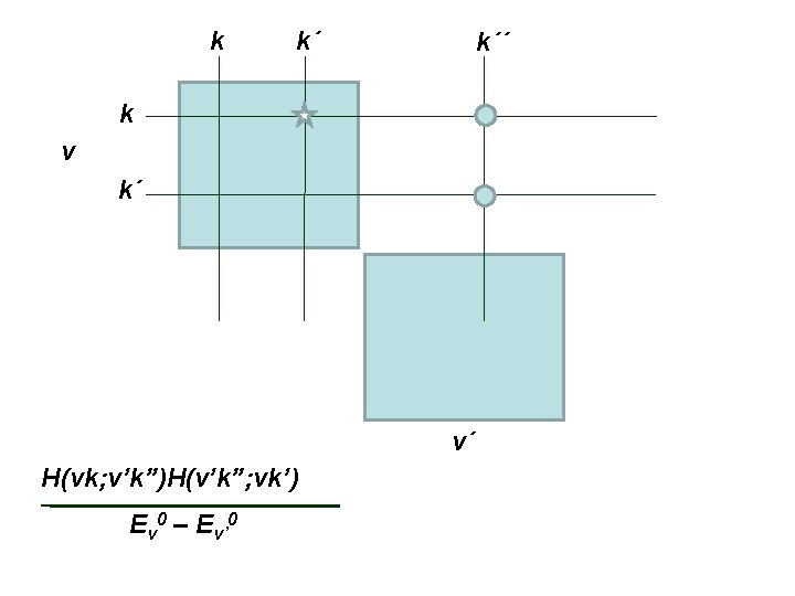
2 nd order perturbation theory expression for new matrix elements One vibrational block (labeled v) H(vk; vk’) + rotational levels ΣΣ v’≠v k” H(vk; v’k”)H(v’k”; vk’) Ev 0 – Ev’ 0 Energy difference approximated to vibrational energy difference of v and v’ Off diagonal MEs removed to 2 nd order. Usual 2 nd order pert theory has k=k´

2 nd order perturbation theory expression for new matrix elements One vibrational block (labeled v) H(vk; vk’) + rotational levels ΣΣ v’≠v k” H(vk; v’k”)H(v’k”; vk’) Ev 0 – Ev’ 0 Energy difference approximated to vibrational energy difference of v and v’ Consider this as the (vk; vk’) element of a TRANSFORMED Hamiltonian

The MEs of the transformed Hamiltonian ~ H(vk; vk’) = H(vk; vk’) + ΣΣ v’≠v k” H(vk; v’k”)H(v’k”; vk’) Ev 0 – Ev’ 0 The second, third, fourth, … perturbation theory expressions can be elegantly formulated using successive contact transformations. See pages 347 to 356 of BJ 1

The contact transformed rot-vib Hamiltonian ~ Hrv = U Hrv U-1 Write U = eiλS = 1 + iλS + (½!)λ 2 S 2 + … where U is unitary and S is a Hermitian operator ~ Hrv has same eigenvalues as Hrv = (H 20+H 02) + λ(H 30+H 21+H 12) + λ 2(H 40+H 31+H 22) + …, = H 0 + λH 1 + λ 2 H 2 + …, Substitute Hrv and U into top equation. Arrange The result in powers of λ to give: ~ ~ 2 Hrv = H 0 + λH 1 + λ H 2 + …,

~ ~ 2 Hrv = H 0 + λH 1 + λ H 2 + …, ~ H 0 = H 0 (= H 20 + H 02 = HO + RR), ~ H 1 = H 1 + i[S, H 0], ~ H 2 = H 2 + i[S, H 1] - ½[S, H 0]], etc. ~ Chose S so that <v´|H 1|v> = 0

~ Starting with Hrv we now make a further ~ contact transformation so that <v´|H 2|v> vanishes. . . and so on as one pleases. This gives the TRANSFORMED Hamiltonian

Hrv = (H 20+H 02) + λ(H 30+H 21+H 12) + λ 2(H 40+H 31+H 22) + …, where Hmn = (Pr , Qr)m(Jα)n Can write the rot-vib Hamiltonian as Hrv = ∞ 2 Σ Σ Hmn m=0 n=0 (only terms up to J 2)

αβQ Q + … μαβe + Σr arαβQr + Σ b rs r s rs Σ ζr, sαQr. Ps rs Hrv = Σμαβ (JαJβ-2 Jαpβ-pαpβ) ΣP r + Σ λr Qr 2 + Σ Φrst Qr. Qs. Qt 2+ 1 2 1 2 H 30 1 6 H 20 + 1 24 Σ Φrstu Qr. Qs. Qt. Qu + … Sum of terms each of which can be symbolically written: Hmn = (Pr , Qr)m(Jα)n - ½ μαβe pαpβ = ½ Σμααe. Jα 2 - ½ μαβe Σrstu ζr, sαζt, uβQr. Ps. Qt. Pu H 02 H 40

Hrv = (H 20+H 02) + λ(H 30+H 21+H 12) + λ 2(H 40+H 31+H 22) + …, where Hmn = (Pr , Qr)m(Jα)n Can write the rot-vib Hamiltonian as Hrv = ∞ 2 Σ Σ Hmn m=0 n=0 (only terms up to J 2) The contact transformed Hamiltonian is ∞ ~ Hrv = Σ ∞ ~ Σ Hmn m=0 n=0 Symmetry allows only an even number of P and J in any one term.

The EFFECTIVE rotational Hamiltonian ~ ~ Hrot = <v|Hrv|v> The WATSONIAN is an (even) power series in The rotational angular momentum operators Jα For a diatomic molecule (in cm-1): Frot = Erot/hc =Bv. J^2 – Dv. J^4 + Hv. J^6 +… Bv = Be –α(v+½)+…, etc. Spectroscopists determine rot-vib constants

Using the effective rotational Hamiltonian in a fitting to data. The theoretician has an easy time of it (in principle) going from Hrv (involving atomic masses, equi geom and VN ) to Erv. The experimentalist has a hard time going from observed ΔErv to rotation-vibration constants in Erot and then to equi geom and VN.

THE EFFECTIVE ROTATIONAL HAMILTONIAN Hrv → ~ Hrv U-1 → ~ Hrot ~ <v|Hrv|v> → Erot

THE EFFECTIVE ROTATIONAL HAMILTONIAN Hrv → ~ Hrv U-1 → ~ Hrot → Erot ~ <v|Hrv|v> BUT It is not always possible to determine all of the parameters in Erot. Indeterminancy is an unavoidable result of the contact transformations. Must chose ~ contact transformation so that Hrot has only determinable parameters.

THE REDUCED ROTATIONAL HAMILTONIAN Hrv → ~ Hrv U-1 → ~ Hrot ~ <v|Hrv|v> → ~ Hrotreduced From special U Hrv U-1 The application of a contact transformation to impose selected constraints on the parameters is called a REDUCTION of the Hamiltonian.

For a diatomic molecule the Watsonian (in cm-1): Frot = Erot/hc =Bv J 2 – Dv J 4 + Hv. J 6 +… For a nonplanar asymmetric top 2 Bs but only 5 Ds General expression has 6 Ds See Watson, JCP 46, 1935 (1967) and pp 347 -356 of BJ 1.

Zeroth order rotational Hamiltonian can be written in general in terms of the six elements of the μ tensor (xx, xy, xz, yy, yz, and zz). But rotating axes to be principal axes gives only three terms (xx, yy, and zz). Only three parameters needed to fit the data.