7 0 Sampling 7 1 The Sampling Theorem
")


 – x(t) uniquely specified by its samples")
 – if ωs ≤ 2 ωM spectrum")

 0 1 2 3 4 5")


 0 1 2")
 x(t) T 1 x(t) T t t T")
 0 0")


=cos ω0 t – sampled at sampling frequency reconstructed")
=cos ω0 t – when aliasing occurs, the original")
=cos ω0 t – many xr(t) exist such that")
")
=cos (ω0 t + Φ) – (a) (b) (c)")


![7. 2 Discrete-time Processing of Continuous-time Signals l Processing continuous-time signals digitally xd[n]=xc(n. T)](https://slidetodoc.com/presentation_image_h2/6244d993da75f66a3381959ad9566cab/image-50.jpg "7. 2 Discrete-time Processing of Continuous-time Signals l Processing continuous-time signals digitally xd[n]=xc(n. T)")
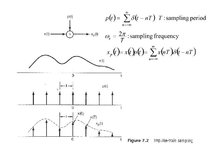
 impulse train sampling with sampling period T (2)")

 – discrete-time (5. 9)")
 See Fig. 7. 22,")
 is a frequency-scaled")
 mapping a sequence to an impulse train (2)")

![h(t) x[n] h[n] y(t) Recovery](https://slidetodoc.com/presentation_image_h2/6244d993da75f66a3381959ad9566cab/image-59.jpg "h(t) x[n] h[n] y(t) Recovery")


=xc(t-∆) – discrete-time equivalent See Fig. 7. 29, p. 543")


")
")
")

 000")
 sampling 0 0 1 2 3 0")
 Aliasing Effect 0")


![Impulse Train Sampling of Discrete-time Signals l Interpolation – h[n] : impulse response of](https://slidetodoc.com/presentation_image_h2/6244d993da75f66a3381959ad9566cab/image-83.jpg "Impulse Train Sampling of Discrete-time Signals l Interpolation – h[n] : impulse response of")


")
")
 l Time Expansion If n/k is an integer, k:")


![Examples • Example 7. 4/7. 5, p. 548, p. 554 of text sampling x[n]](https://slidetodoc.com/presentation_image_h2/6244d993da75f66a3381959ad9566cab/image-99.jpg "Examples • Example 7. 4/7. 5, p. 548, p. 554 of text sampling x[n]")


 yes : inserting one zero after")
 no : inserting one zero after")


- Slides: 112
7. 0 Sampling 7. 1 The Sampling Theorem A link between Continuous-time/Discrete-time Systems x(t) y(t) Sampling x[n] y[n] h(t) x[n]=x(n. T), T : sampling period h(t) x[n] h[n] y[n] Recovery y(t)
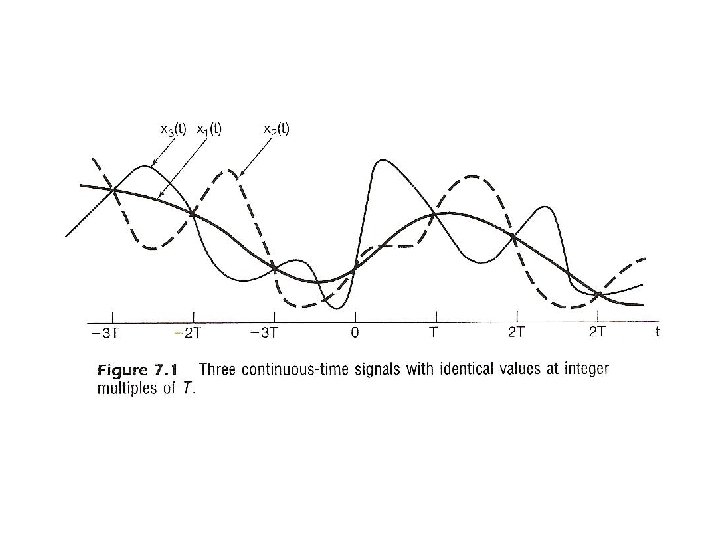
Motivation: handling continuous-time signals/systems digitally using computing environment – accurate, programmable, flexible, reproducible, powerful – compatible to digital networks and relevant technologies – all signals look the same when digitized, except at different rates, thus can be supported by a single network Question: under what kind of conditions can a continuous-time signal be uniquely specified by its discrete-time samples? See Fig. 7. 1, p. 515 of text – Sampling Theorem
Recovery from Samples ? 0 1 2
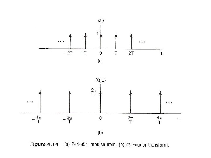
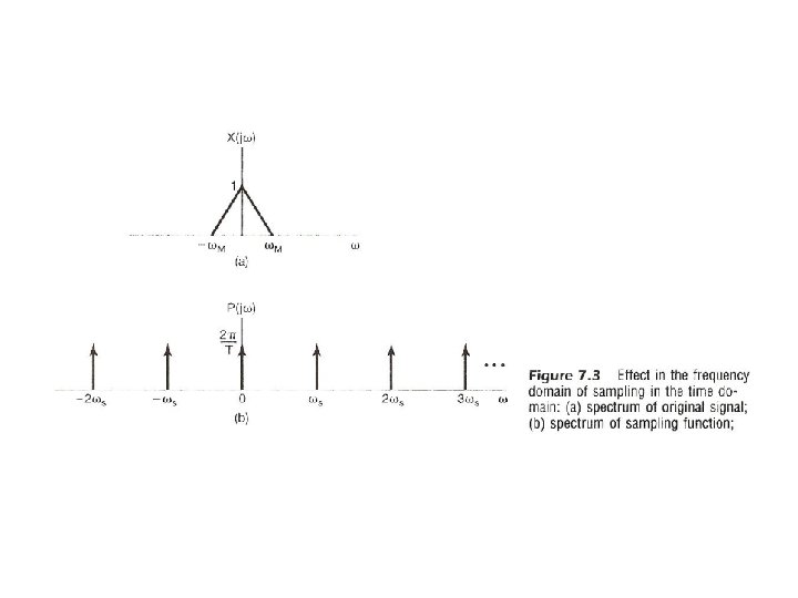
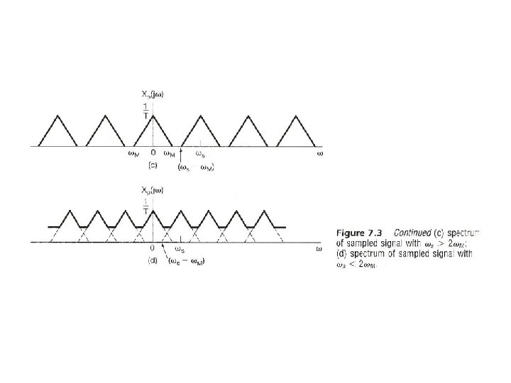
Impulse Train Sampling See Fig. 4. 14, p. 300 of text – periodic spectrum, superposition of scaled, shifted replicas of X(jω) See Fig. 7. 3, p. 517 of text
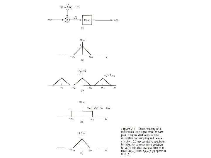
Impulse Train Sampling l Sampling Theorem (1/2) – x(t) uniquely specified by its samples x(n. T), n=0, 1, 2…… – precisely reconstructed by an ideal lowpass filter with Gain T and cutoff frequency ωM < ωc < ωs- ωM applied on the impulse train of sample values See Fig. 7. 4, p. 519 of text
Impulse Train Sampling l Sampling Theorem (2/2) – if ωs ≤ 2 ωM spectrum overlapped, frequency components confused --- aliasing effect can’t be reconstructed by lowpass filtering See Fig. 7. 3, p. 518 of text
Aliasing Effect 000
Continuous/Discrete Sinusoidals (p. 36 of 1. 0) 0 1 2 3 4 5
Sampling sampling 0 0 1 2 3 0
Aliasing Effect 0
Sampling Thm 0 0
Recovery from Samples ? (p. 3 of 7. 0) 0 1 2
Practical Sampling (any other pulse shape) x(t) T 1 x(t) T t t T t 0 0 0 t
Practical Sampling (any other pulse shape) 0 0
Impulse Train Sampling l Practical Issues – nonideal lowpass filters accurate enough for practical purposes determined by acceptable level of distortion oversampling ωs = 2 ωM + ∆ ω �� – sampled by pulse train with other pulse shapes – signals practically not bandlimited : pre-filtering
Oversampling with Non-ideal Lowpass Filters 0 0
Signals not Bandlimited 0 0
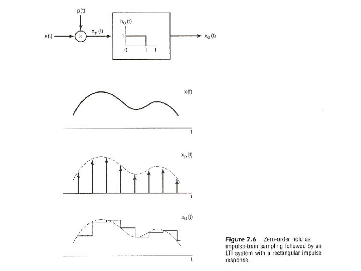
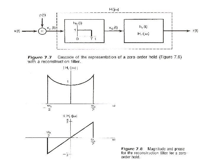
Sampling with A Zero-order Hold l Zero-order Hold: – holding the sampled value until the next sample taken – modeled by an impulse train sampler followed by a system with rectangular impulse response l Reconstructed by a lowpass filter Hr(jω) See Fig. 7. 6, 7. 7, 7. 8, p. 521, 522 of text
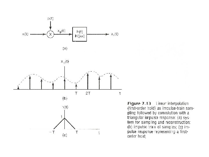
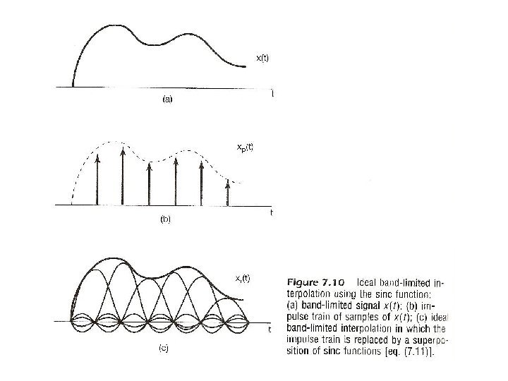
Interpolation l Impulse train sampling/ideal lowpass filtering See Fig. 7. 10, p. 524 of text
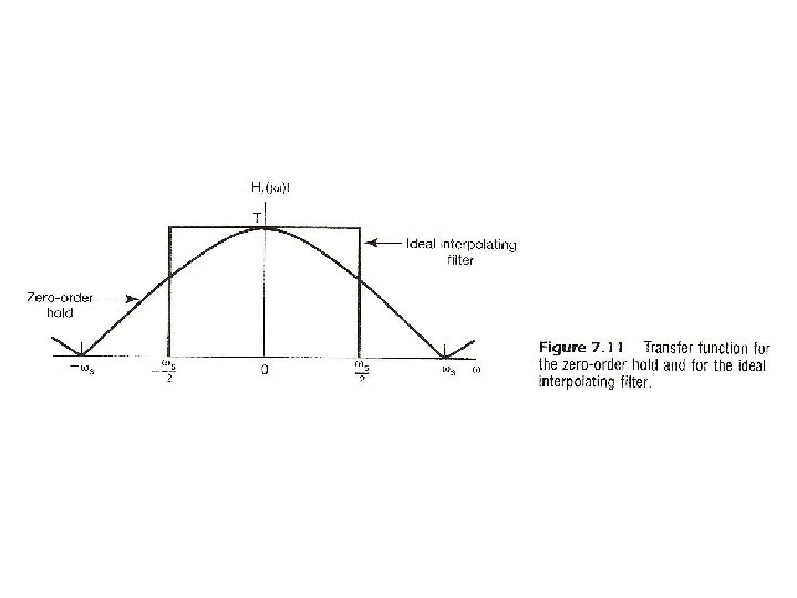
Ideal Interpolation
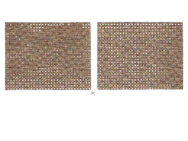
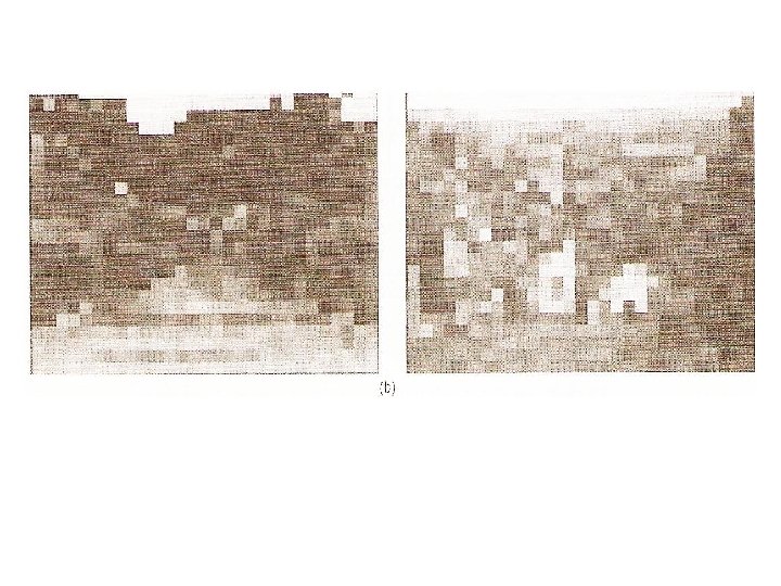
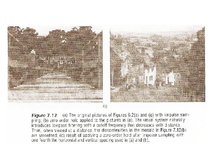
Interpolation l Zero-order hold can be viewed as a “coarse” interpolation See Fig. 7. 11, p. 524 of text l Sometimes additional lowpass filtering naturally applied e. g. viewed at a distance by human eyes, mosaic smoothed naturally See Fig. 7. 12, p. 525 of text
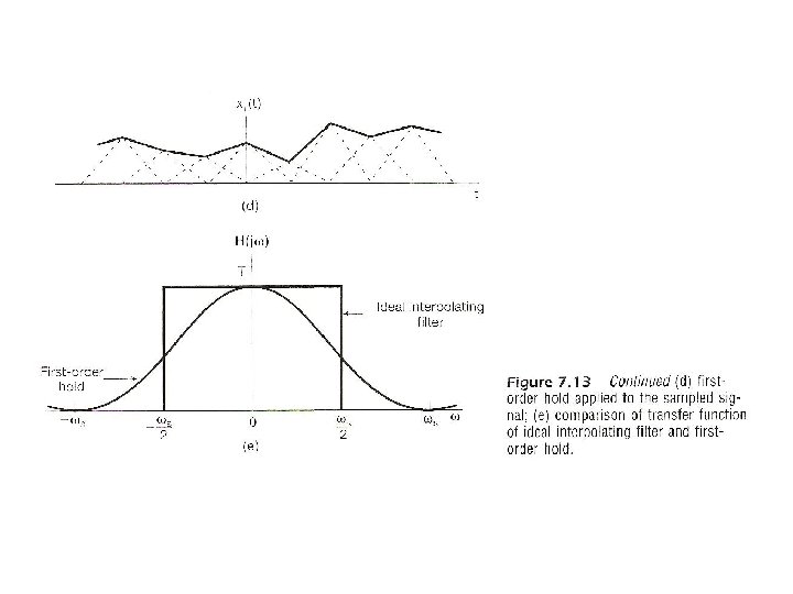
Interpolation l Higher order holds – zero-order : output discontinuous – first-order : output continuous, discontinuous derivatives See Fig. 7. 13, p. 526, 527 of text – second-order : continuous up to first derivative discontinuous second derivative
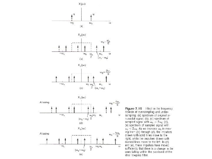
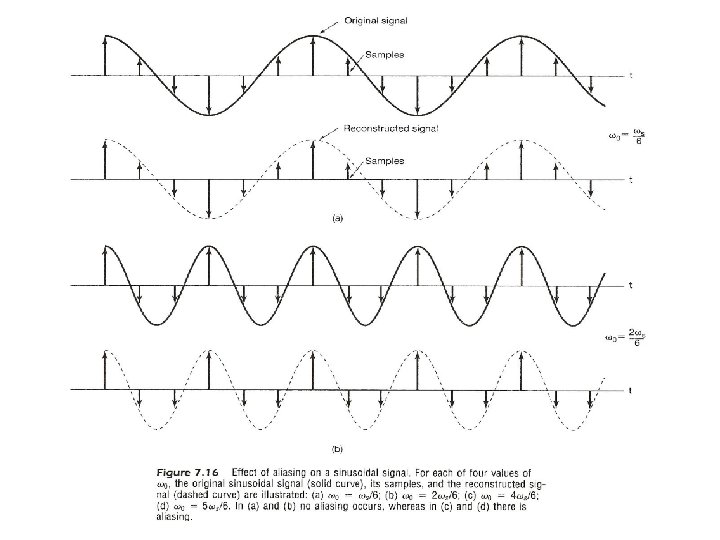
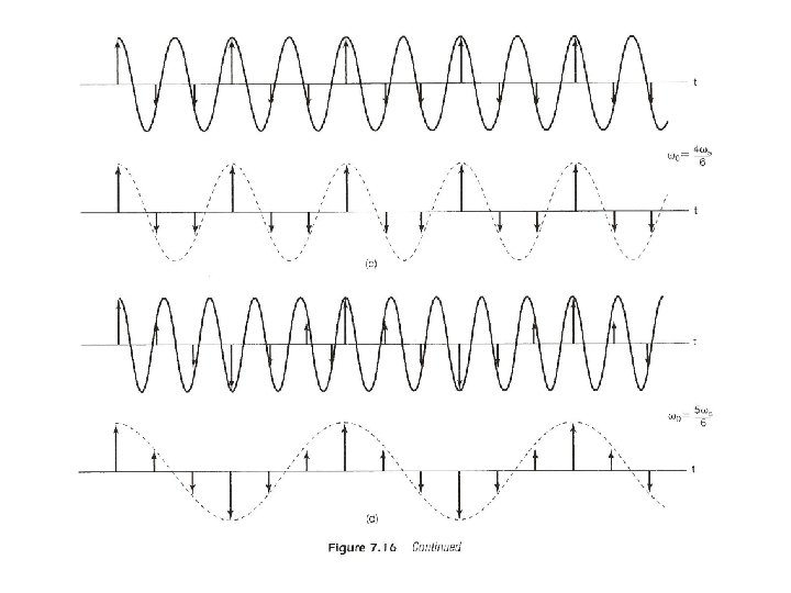
Aliasing l Consider a signal x(t)=cos ω0 t – sampled at sampling frequency reconstructed by an ideal lowpass filter with xr(t) : reconstructed signal fixed ωs, varying ω0
Aliasing l Consider a signal x(t)=cos ω0 t – when aliasing occurs, the original frequency ω0 takes on the identity of a lower frequency, ωs – ω0 – w 0 confused with not only ωs + ω0, but ωs – ω0 See Fig. 7. 15, 7. 16, p. 529 -531 of text
Aliasing l Consider a signal x(t)=cos ω0 t – many xr(t) exist such that the problem is it is not easy to find the right one – if x(t) = cos(ω0 t + ϕ) the impulses have extra phases ejϕ, e-jϕ –
Sinusoidals (p. 25 of 4. 0)
Aliasing l Consider a signal x(t)=cos (ω0 t + Φ) – (a) (b) (c) (d) phase also changed
Example 7. 1 of Text Sampling is “timevarying” 0 0 0
Example 7. 1 of Text 0 0 0
Example 7. 1 of Text
Examples • Example 7. 1, p. 532 of text (Problem 7. 39, p. 571 of text) sampled and low-pass filtered
7. 2 Discrete-time Processing of Continuous-time Signals l Processing continuous-time signals digitally xd[n]=xc(n. T) xc(t) C/D Conversion D/A Converter h(t) x[n] h[n] yc(t) D/C Conversion Discrete-time System A/D Converter x(t) yd[n]=yc(n. T) y[n] Recovery y(t)
Formal Formulation/Analysis l C/D Conversion (1) impulse train sampling with sampling period T (2) mapping the impulse train to a sequence with unity spacing – normalization (or scaling) in time
Formal Formulation/Analysis l Frequency Domain Representation ω for continuous-time, Ω for discrete-time, only in this section
Formal Formulation/Analysis l Frequency Domain Relationships – continuous-time (4. 9) – discrete-time (5. 9)
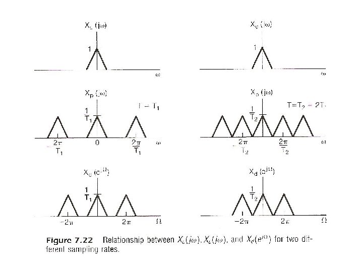
Formal Formulation/Analysis l Frequency Domain Relationships – relationship (7. 6) See Fig. 7. 22, p. 537 of text
C/D Conversion 0 0 1 2 3 4 1 – Xd(ejΩ) is a frequency-scaled (by T) version of Xp(jω) xd[n] is a time-scaled (by 1/T) version of xp(t) – Xd(ejΩ) periodic with period 2π Xp(jω) periodic with period 2π/T=ωs
Formal Formulation/Analysis l D/C Conversion (1) mapping a sequence to an impulse train (2) lowpass filtering
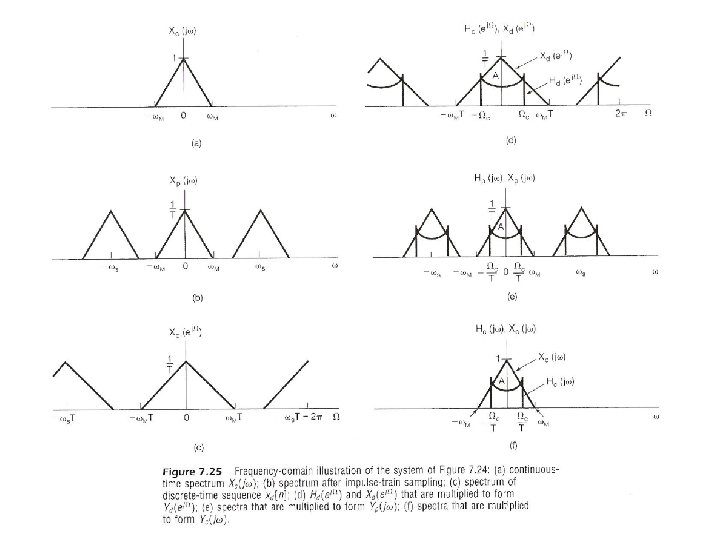
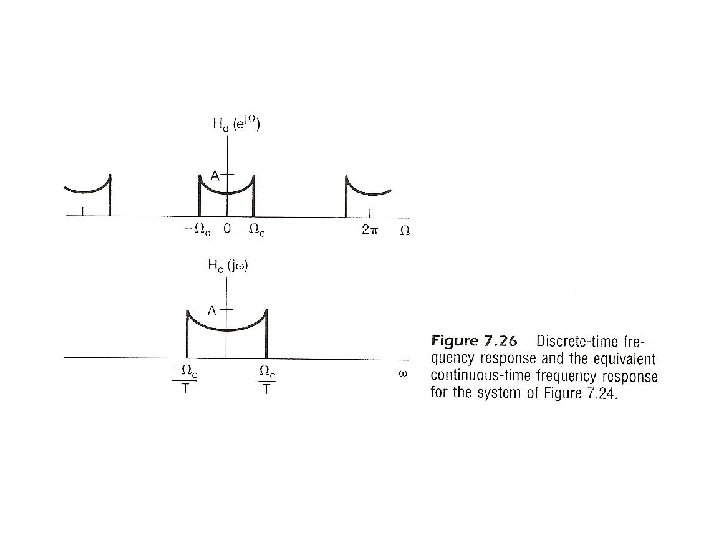
Formal Formulation/Analysis l Complete System See Fig. 7. 24, 7. 25, 7. 26, p. 538, 539, 540 of text equivalent to a continuous-time system if the sampling theorem is satisfied (7. 24 ) (7. 25 )
h(t) x[n] h[n] y(t) Recovery
Discrete-time Processing of Continuous-time Signals l Note – the complete system is linear and time-invariant if the sampling theorem is satisfied – sampling process itself is NOT time-invariant
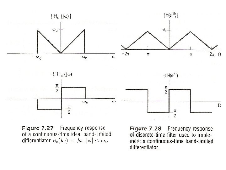
Examples l Digital Differentiator – band-limited differentiator – discrete-time equivalent See Fig. 7. 27, 7. 28, p. 541, 542 of text
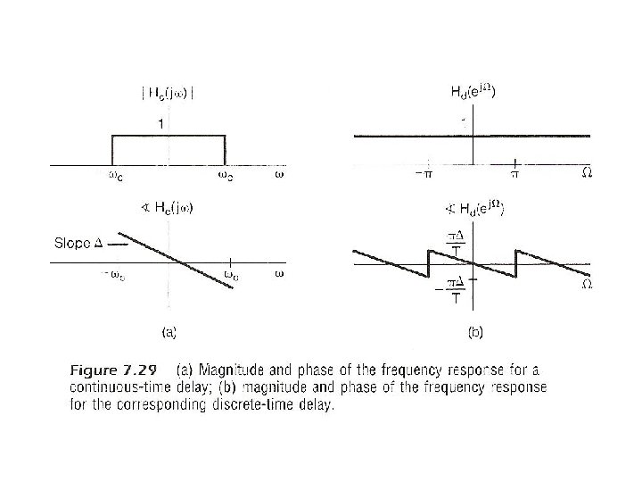
Examples l Delay – yc(t)=xc(t-∆) – discrete-time equivalent See Fig. 7. 29, p. 543 of text
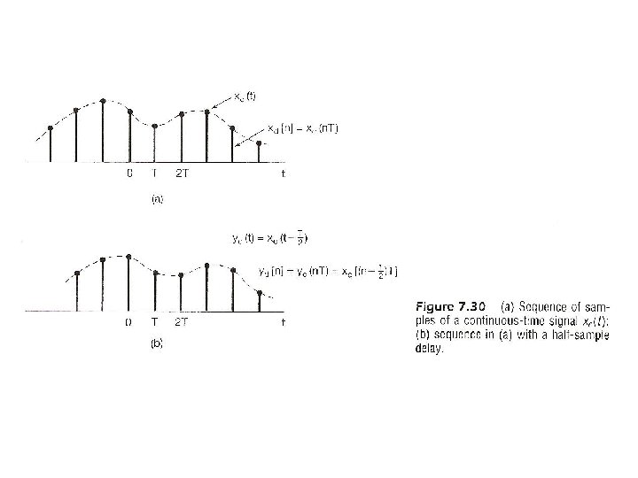
Examples l Delay – ∆/T an integer – ∆/T not an integer undefined in principle but makes sense in terms of sampling if the sampling theorem is satisfied e. g. ∆/T=1/2, half-sample delay See Fig. 7. 30, p. 544 of text
7. 3 Change of Sampling Frequency Up/Down Sampling 0 0 0 Up Sampling Down Sampling
Impulse Train Sampling of Discrete-time Signals l Completely in parallel with impulse train sampling of continuous-time signals See Fig. 7. 31, p. 546 of text
See Fig. 7. 31, p. 546 of text
(P. 5 of 7. 0)
(P. 7 of 7. 0)
(P. 8 of 7. 0)
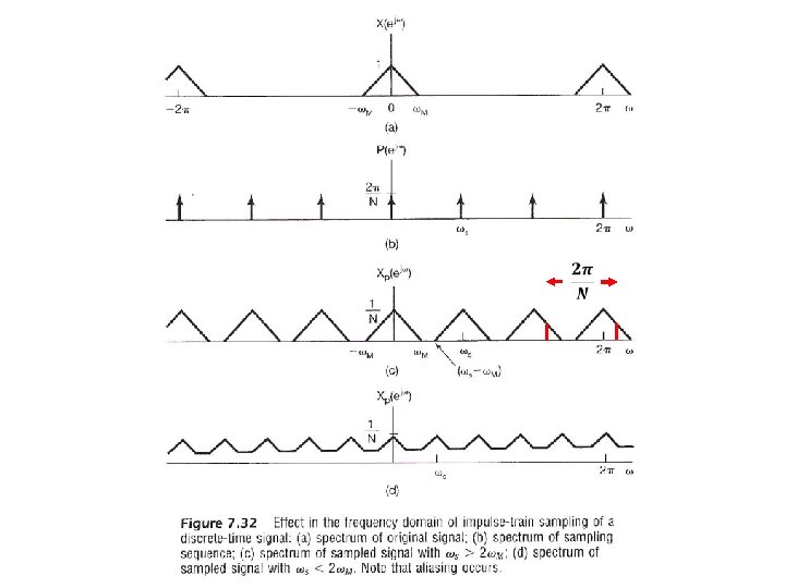
Impulse Train Sampling of Discrete-time Signals l Completely in parallel with impulse train sampling of continuous-time signals See Fig. 7. 32, p. 547 of text
Aliasing Effect (P. 13 of 7. 0) 000
Sampling (P. 15 of 7. 0) sampling 0 0 1 2 3 0
Aliasing Effect (P. 16 of 7. 0) Aliasing Effect 0
Aliasing for Discrete-time Signals
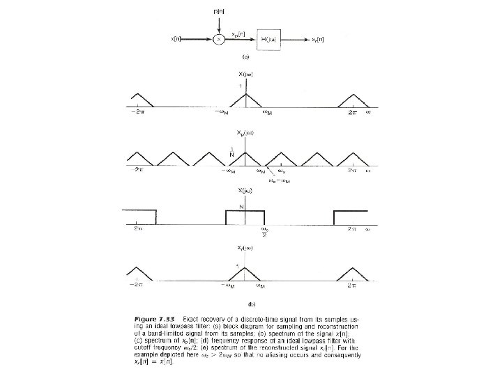
Impulse Train Sampling of Discrete-time Signals l Completely in parallel with impulse train sampling of continuous-time signals See Fig. 7. 33, p. 548 of text – ωs < 2ωM, aliasing occurs filter output but xr[n] ≠ x[n] xr[k. N] = x[k. N], k=0, ± 1, ± 2, ……
Impulse Train Sampling of Discrete-time Signals l Interpolation – h[n] : impulse response of the lowpass filter – in general a practical filter hr[n] is used
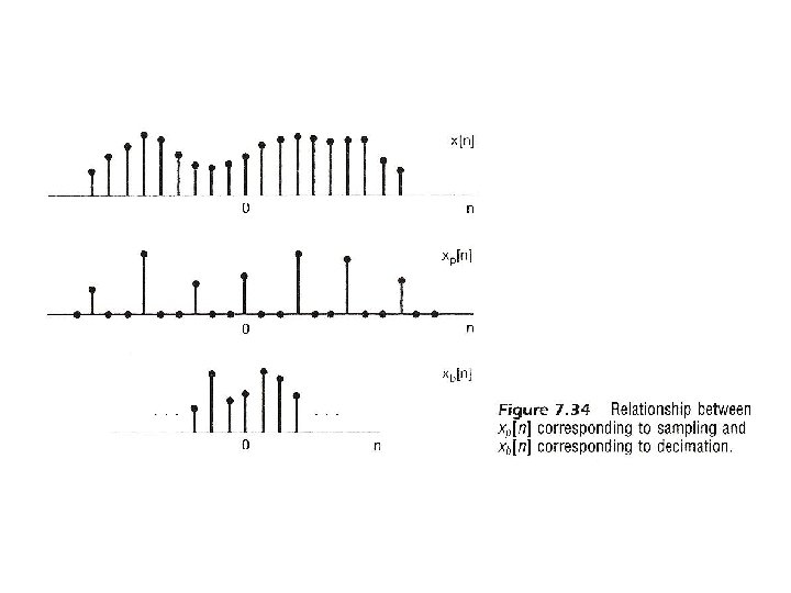
Decimation/Interpolation l Decimation: reducing the sampling frequency by a factor of N, downsampling : two reversible steps – taking every N-th sample, leaving zeros in between – deleting all zero’s between non-zero samples to produce a new sequence (inverse of time expansion property of discrete-time Fourier transform) – both steps reversible in both time/frequency domains See Fig. 7. 34, p. 550 of text
(p. 38 of 5. 0)
(p. 39 of 5. 0)
(p. 37 of 5. 0) l Time Expansion If n/k is an integer, k: positive integer See Fig. 5. 13, p. 377 of text See Fig. 5. 14, p. 378 of text
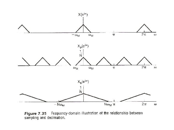
Decimation/Interpolation l Decimation: See Figs. 7. 34, 7. 35, p. 550, 551 of text
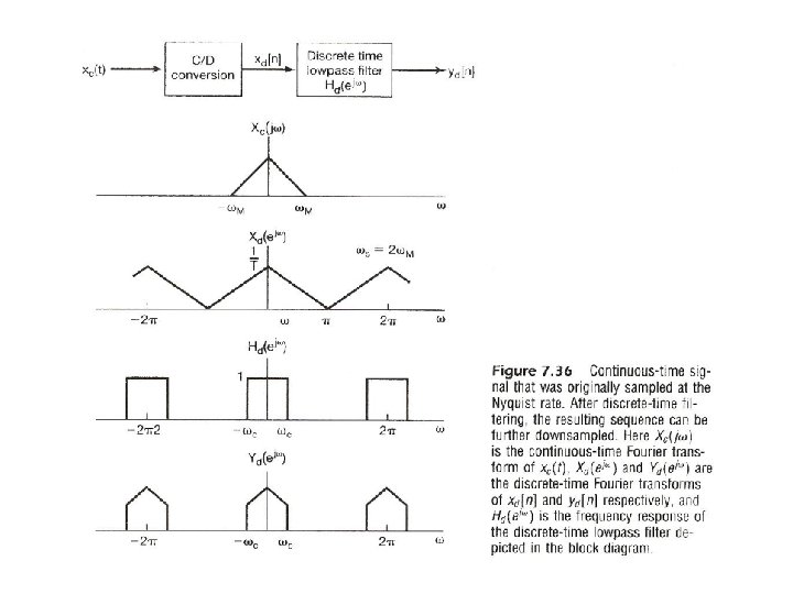
Decimation/Interpolation l Decimation – decimation without introducing aliasing requires oversampling situation See an example in Fig. 7. 36, p. 552 of text
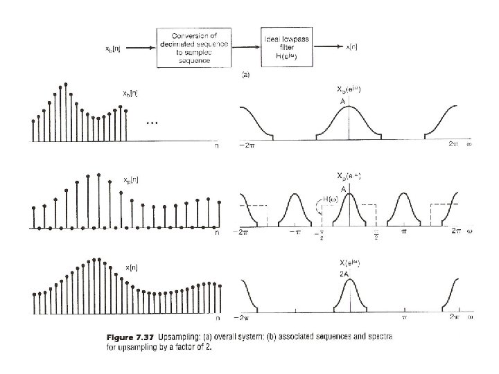
Decimation/Interpolation l Interpolation: increasing the sampling frequency by a factor of N, upsampling – reverse the two-step process in decimation from xb[n] construct xp[n] by inserting N-1 zero’s from xp[n] construct x[n] by lowpass filtering See Fig. 7. 37, p. 553 of text l Change of sampling frequency by a factor of N/M: first interpolating by N, then decimating by M
Decimation/Interpolation 0 012 Interpolation Decimation 012
Decimation/Interpolation 0 0 0
Examples • Example 7. 4/7. 5, p. 548, p. 554 of text sampling x[n] without aliasing
Examples • Example 7. 4/7. 5, p. 548, p. 554 of text maximum possible downsampling: using full band [-π, π]
Examples • Example 7. 4/7. 5, p. 548, p. 554 of text
Problem 7. 6, p. 557 of text
Problem 7. 20, p. 560 of text : inserting one zero after each sample : decimation 2: 1, extracting every second sample Which of (a)(b) corresponds to low-pass filtering with ?
Problem 7. 20, p. 560 of text (a) yes : inserting one zero after each sample : decimation 2: 1, extracting every second sample
Problem 7. 20, p. 560 of text (b) no : inserting one zero after each sample : decimation 2: 1, extracting every second sample
Problem 7. 23, p. 562 of text
Problem 7. 23, p. 562 of text
Problem 7. 23, p. 562 of text
Problem 7. 24, p. 562 of text 2
Problem 7. 41, p. 572 of text
Problem 7. 41, p. 572 of text
Problem 7. 52, p. 580 of text dual problem for frequency domain sampling