Lecture 17 Final Project Design your own survey

Lecture 17

Final Project • Design your own survey! – Find an interesting question and population – Design your sampling plan – Collect Data – Analyze using R • Write 5 page paper on your results • Due April 21

Final presentation • During the last class (April 26) all students will be required to give a short presentation – Select one of the three projects – Make a powerpoint presentation (no more than 35 slides) – Present your results to the class

Final Project • Design your own survey! – Find an interesting question and population – Design your sampling plan – Collect Data – Analyze using R • Write 5 page paper on your results • Due December 1

Final presentation • All are required to give a short presentation • Last two classes (December 1 and 6) – Select one of the three projects – Make a powerpoint presentation (no more than 35 slides) – Present your results to the class

Statistics • Main ideas of statistics – Given multiple plausible models select one (or several) that is (are) the most consistent with the observed data – Quantify a measure of belief in our solution • The main idea is that if something looks like a very unlikely coincidence we would prefer another more likely explanation

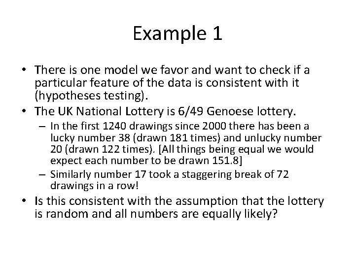
Example 1 • There is one model we favor and want to check if a particular feature of the data is consistent with it (hypotheses testing). • The UK National Lottery is 6/49 Genoese lottery. – In the first 1240 drawings since 2000 there has been a lucky number 38 (drawn 181 times) and unlucky number 20 (drawn 122 times). [All things being equal we would expect each number to be drawn 151. 8] – Similarly number 17 took a staggering break of 72 drawings in a row! • Is this consistent with the assumption that the lottery is random and all numbers are equally likely?

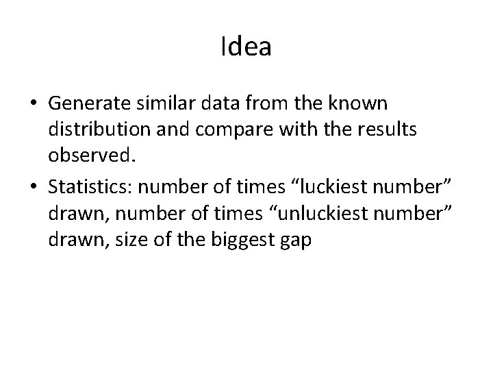
Idea • Generate similar data from the known distribution and compare with the results observed. • Statistics: number of times “luckiest number” drawn, number of times “unluckiest number” drawn, size of the biggest gap

R simulation • Code Loterry 1240. R • What is our conclusion?

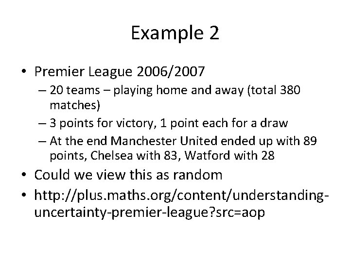
Example 2 • Premier League 2006/2007 – 20 teams – playing home and away (total 380 matches) – 3 points for victory, 1 point each for a draw – At the end Manchester United ended up with 89 points, Chelsea with 83, Watford with 28 • Could we view this as random • http: //plus. maths. org/content/understandinguncertainty-premier-league? src=aop

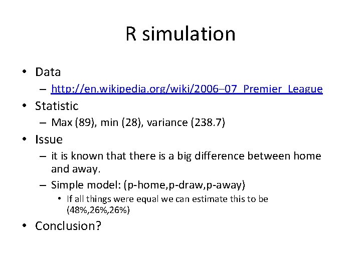
R simulation • Data – http: //en. wikipedia. org/wiki/2006– 07_Premier_League • Statistic – Max (89), min (28), variance (238. 7) • Issue – it is known that there is a big difference between home and away. – Simple model: (p-home, p-draw, p-away) • If all things were equal we can estimate this to be (48%, 26%) • Conclusion?

Other issues • In sports – successive trials are probably not independent • Can we test this? What would we need? – Data – Statistics (numerical measurement that caries information about the feature we are interested in) – Simulation scheme/model

Other statistical problems • Having several models and deciding how likely each model is given data. • Bayesian statistics – Need prior believe in each model – Update the believe based on data

Deciding between several models • One option is to use Bayesian approach

Bayesian statistics • A method for updating and combining information expressed in terms of probabilities (data and prior believes) • Recent notable uses – Nate Silver http: //fivethirtyeight. com – Search for Air France Flight 447 http: //en. wikipedia. org/wiki/Air_France_Flight_4 47

Example 1: • Testing for disease or drug. – Two models: • Subject has the disease (uses drugs) – Test is positive with probability q 1 (sensitivity) • Subject does not have the disease (is clean) – Test is negative with probability q 2 (specificity) – Prior information • Certain proportion p of the population has the disease

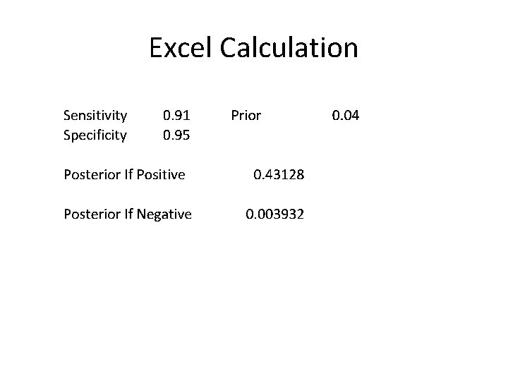
• It is claimed that a Drug. Wipe 5 has sensitivity of 91% and specificity of 95% • About 4% of the population uses • A randomly selected worker tested positive. – What is the chance he is a user? • http: //www. drugwarfacts. org/cms/Drug_Testi ng

Excel Calculation

• A spotter has a 30% success rate in spotting workers who use. A person selected by a spotter was tested positive. Is there a difference? • Comments?

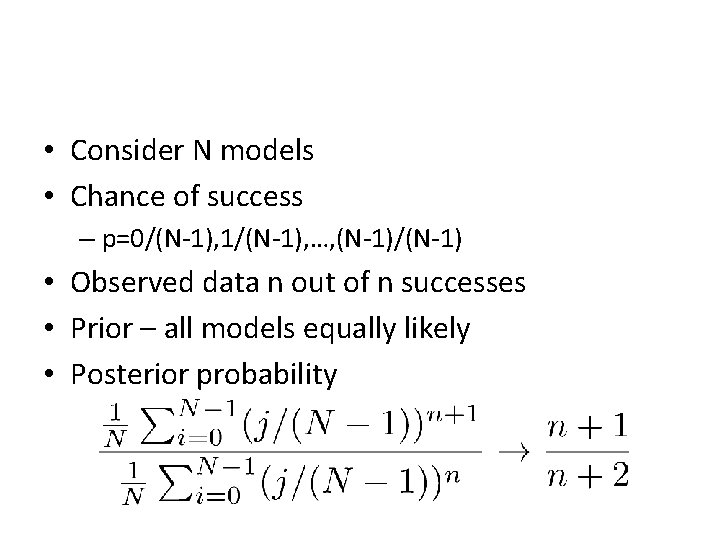
The rule of succession • Derived by Laplace (1814) • We have an experiment that can end up in success or failure • We performed n experiments and all of them were successes. What is the chance that the next one will be success?

• Consider N models • Chance of success – p=0/(N-1), 1/(N-1), …, (N-1)/(N-1) • Observed data n out of n successes • Prior – all models equally likely • Posterior probability

Example 2 b • What if we observed s out of n successes? • Other priors?