Monte Carlo Techniques Basic Concepts Chapter 1314 15

Monte Carlo Techniques Basic Concepts Chapter (13)14, 15 of “Physically Based Rendering” by Pharr&Humphreys 782 1

Reading 13: light sources Read on your own 14. 1: probability Intro, review 14. 2: monte carlo Important basics 14. 3: sampling random variables 14. 4: transforming distributions Basic procedures for sampling 14. 5: 2 D sampling 15. 1: Russian roulette Improve efficiency 15. 2: careful sample placement 15. 3: bias Techniques to reduce variance 15. 4: importance sampling 15. 5: sampling reflection functions 15. 6: sampling light sources 15. 7: volume scattering 782 Sampling graphics 3

Randomized Algorithms • Las Vegas: – Always give right answer, but use elements of randomness on the way – Example: randomized quicksort • Monte Carlo: – stochastic / non-deterministic – give the right answer on average (in the limit) 782 4

Monte Carlo • Efficiency, relative to other algorithms, increases with number of dimensions • For problems such as – integrals difficult to evaluate because of multidimensional, complex boundary conditions (i. e. , no easy closed form solutions) – Those with large number of coupled degrees of freedom 782 5

Monte Carlo Integration • Pick a set of evaluation points • Accuracy grows with O(N-0. 5), i. e. in order to do twice as good we need 4 times as many samples • Artifacts manifest themselves as noise • Research - minimize error while minimizing the number of necessary rays 782 6

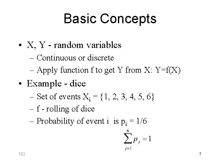
Basic Concepts • X, Y - random variables – Continuous or discrete – Apply function f to get Y from X: Y=f(X) • Example - dice – Set of events Xi = {1, 2, 3, 4, 5, 6} – f - rolling of dice – Probability of event i is pi = 1/6 782 7

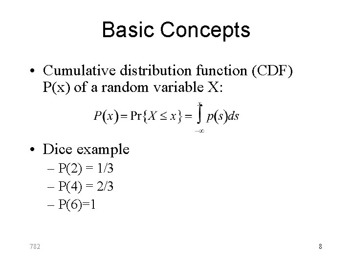
Basic Concepts • Cumulative distribution function (CDF) P(x) of a random variable X: • Dice example – P(2) = 1/3 – P(4) = 2/3 – P(6)=1 782 8

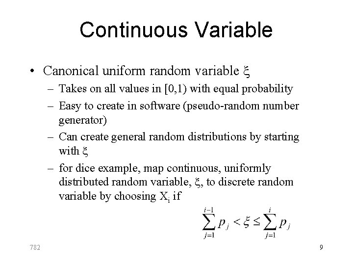
Continuous Variable • Canonical uniform random variable x – Takes on all values in [0, 1) with equal probability – Easy to create in software (pseudo-random number generator) – Can create general random distributions by starting with x – for dice example, map continuous, uniformly distributed random variable, x, to discrete random variable by choosing Xi if 782 9

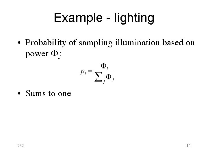
Example - lighting • Probability of sampling illumination based on power Fi: • Sums to one 782 10

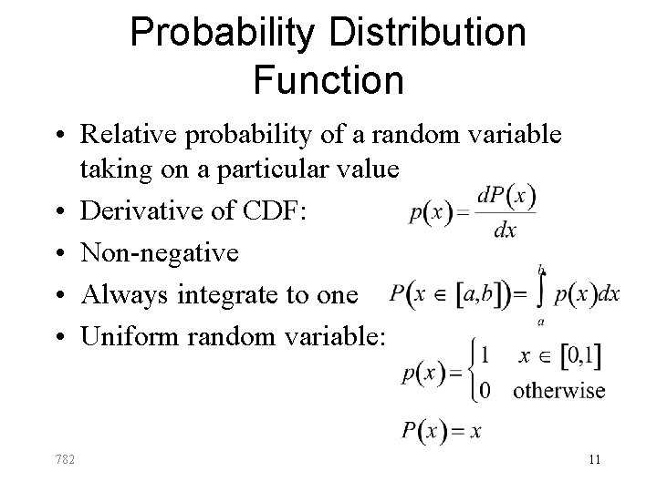
Probability Distribution Function • Relative probability of a random variable taking on a particular value • Derivative of CDF: • Non-negative • Always integrate to one • Uniform random variable: 782 11

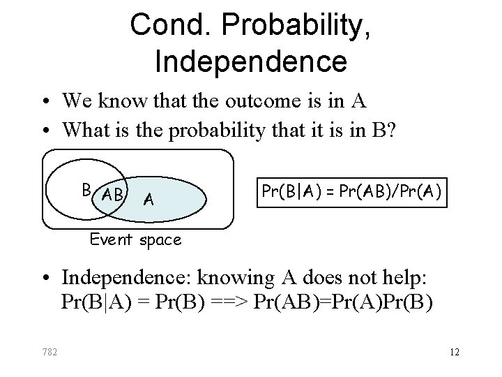
Cond. Probability, Independence • We know that the outcome is in A • What is the probability that it is in B? B AB A Pr(B|A) = Pr(AB)/Pr(A) Event space • Independence: knowing A does not help: Pr(B|A) = Pr(B) ==> Pr(AB)=Pr(A)Pr(B) 782 12

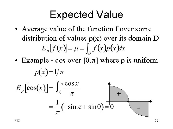
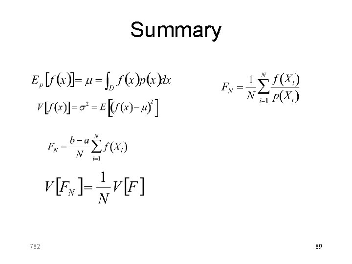
Expected Value • Average value of the function f over some distribution of values p(x) over its domain D • Example - cos over [0, p] where p is uniform + 782 13

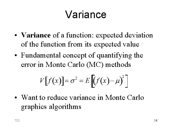
Variance • Variance of a function: expected deviation of the function from its expected value • Fundamental concept of quantifying the error in Monte Carlo (MC) methods • Want to reduce variance in Monte Carlo graphics algorithms 782 14

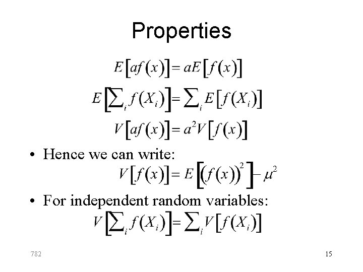
Properties • Hence we can write: • For independent random variables: 782 15

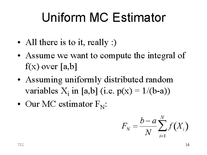
Uniform MC Estimator • All there is to it, really : ) • Assume we want to compute the integral of f(x) over [a, b] • Assuming uniformly distributed random variables Xi in [a, b] (i. e. p(x) = 1/(b-a)) • Our MC estimator FN: 782 16

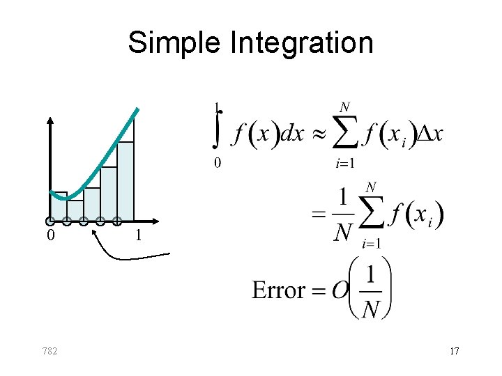
Simple Integration 0 782 1 17

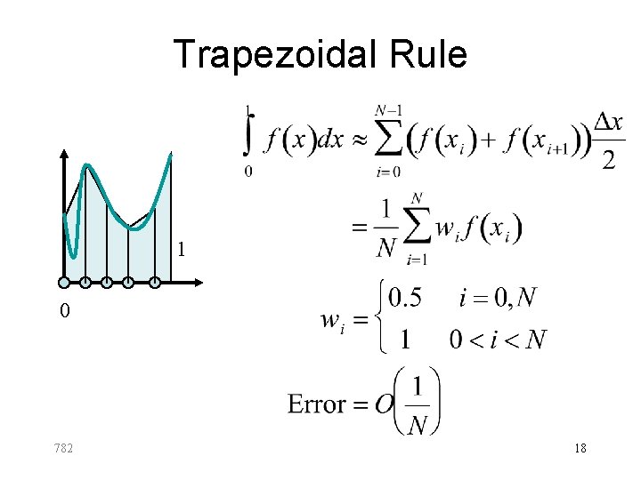
Trapezoidal Rule 1 0 782 18

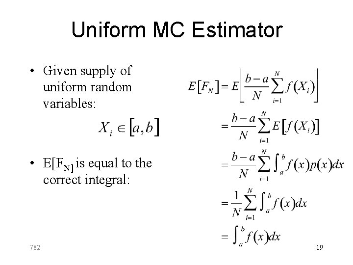
Uniform MC Estimator • Given supply of uniform random variables: • E[FN] is equal to the correct integral: 782 19

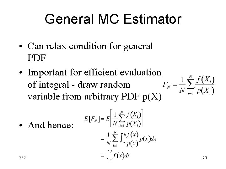
General MC Estimator • Can relax condition for general PDF • Important for efficient evaluation of integral - draw random variable from arbitrary PDF p(X) • And hence: 782 20

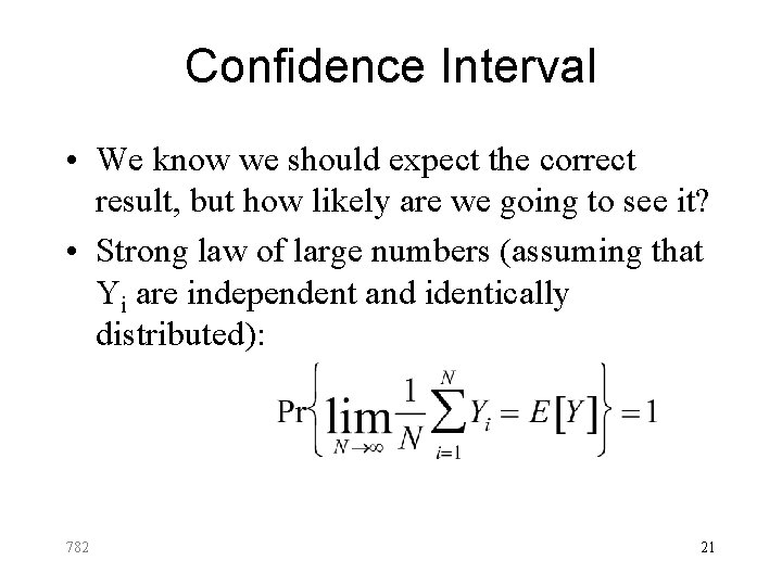
Confidence Interval • We know we should expect the correct result, but how likely are we going to see it? • Strong law of large numbers (assuming that Yi are independent and identically distributed): 782 21

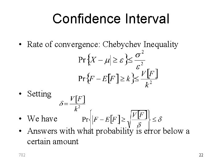
Confidence Interval • Rate of convergence: Chebychev Inequality • Setting • We have • Answers with what probability is error below a certain amount 782 22

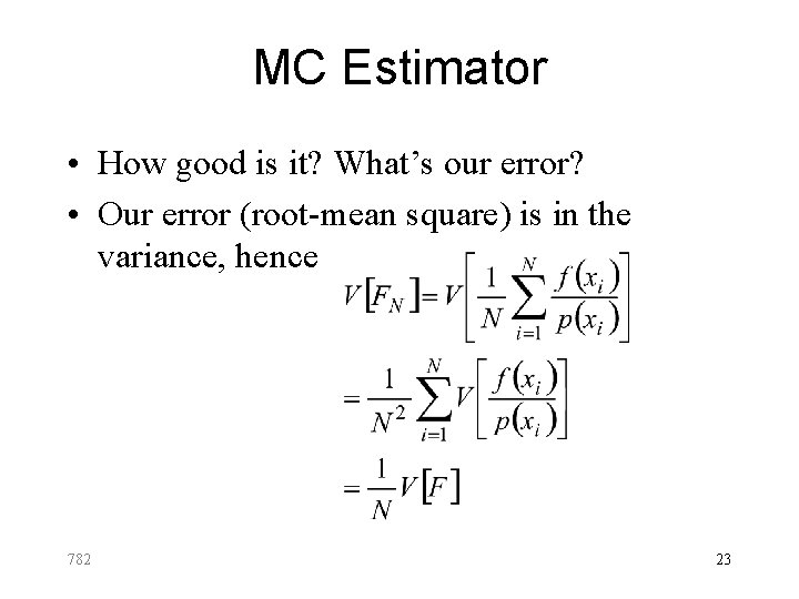
MC Estimator • How good is it? What’s our error? • Our error (root-mean square) is in the variance, hence 782 23

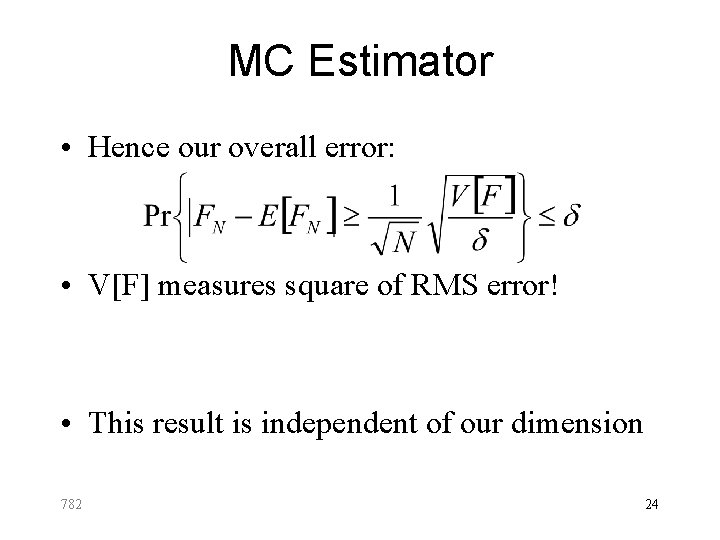
MC Estimator • Hence our overall error: • V[F] measures square of RMS error! • This result is independent of our dimension 782 24

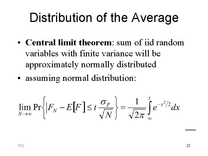
Distribution of the Average • Central limit theorem: sum of iid random variables with finite variance will be approximately normally distributed • assuming normal distribution: 782 25

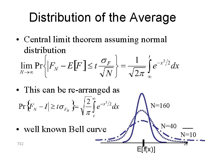
Distribution of the Average • Central limit theorem assuming normal distribution • This can be re-arranged as N=160 N=40 • well known Bell curve 782 N=10 E[f(x)] 26

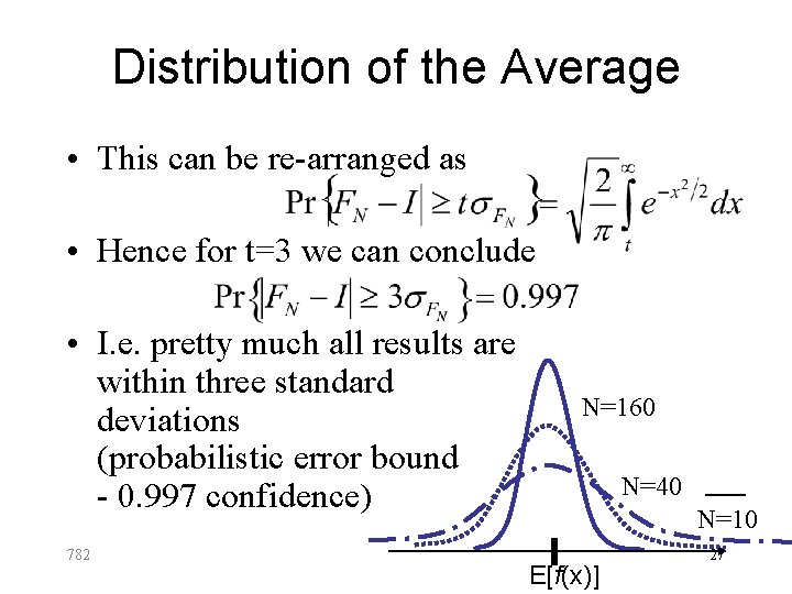
Distribution of the Average • This can be re-arranged as • Hence for t=3 we can conclude • I. e. pretty much all results are within three standard deviations (probabilistic error bound - 0. 997 confidence) 782 N=160 N=40 N=10 E[f(x)] 27

Choosing Samples • How to sample random variables? • Assume we can do uniform distribution • How to do general distributions? – Inversion – Rejection – Transformation 782 28

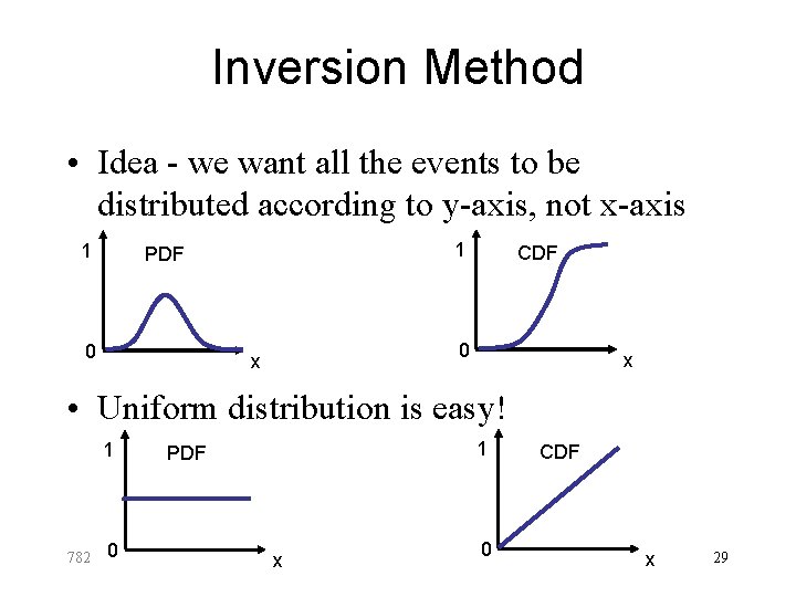
Inversion Method • Idea - we want all the events to be distributed according to y-axis, not x-axis 1 1 PDF 0 CDF 0 x x • Uniform distribution is easy! 1 782 0 1 PDF x 0 CDF x 29

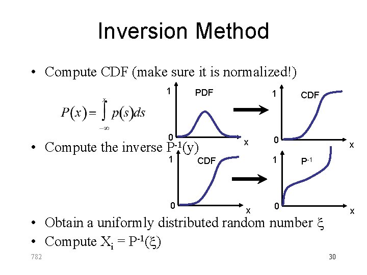
Inversion Method • Compute CDF (make sure it is normalized!) 1 • Compute the inverse PDF 0 P-1(y) 1 0 1 x 0 1 CDF x P-1 0 x • Obtain a uniformly distributed random number x • Compute Xi = P-1(x) 782 30

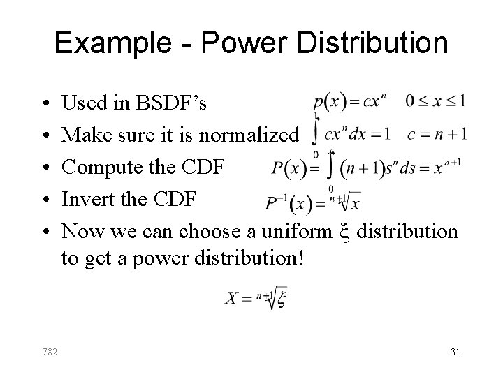
Example - Power Distribution • • • 782 Used in BSDF’s Make sure it is normalized Compute the CDF Invert the CDF Now we can choose a uniform x distribution to get a power distribution! 31

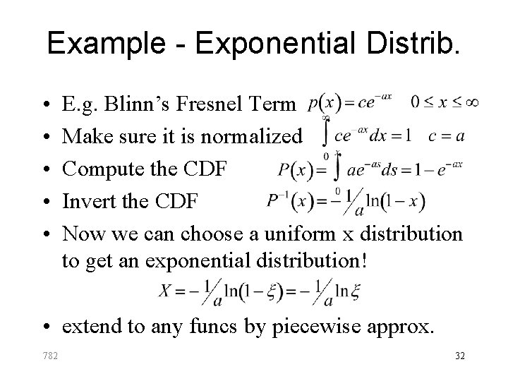
Example - Exponential Distrib. • • • E. g. Blinn’s Fresnel Term Make sure it is normalized Compute the CDF Invert the CDF Now we can choose a uniform x distribution to get an exponential distribution! • extend to any funcs by piecewise approx. 782 32

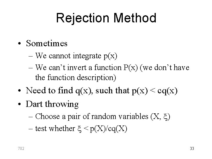
Rejection Method • Sometimes – We cannot integrate p(x) – We can’t invert a function P(x) (we don’t have the function description) • Need to find q(x), such that p(x) < cq(x) • Dart throwing – Choose a pair of random variables (X, x) – test whether x < p(X)/cq(X) 782 33

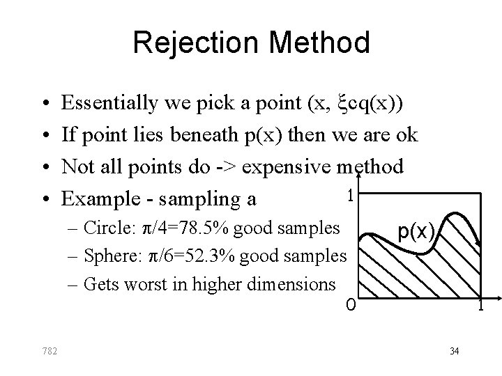
Rejection Method • • Essentially we pick a point (x, xcq(x)) If point lies beneath p(x) then we are ok Not all points do -> expensive method 1 Example - sampling a – Circle: p/4=78. 5% good samples p(x) – Sphere: p/6=52. 3% good samples – Gets worst in higher dimensions 1 0 782 34

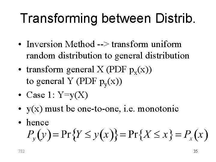
Transforming between Distrib. • Inversion Method --> transform uniform random distribution to general distribution • transform general X (PDF px(x)) to general Y (PDF py(x)) • Case 1: Y=y(X) • y(x) must be one-to-one, i. e. monotonic • hence 782 35

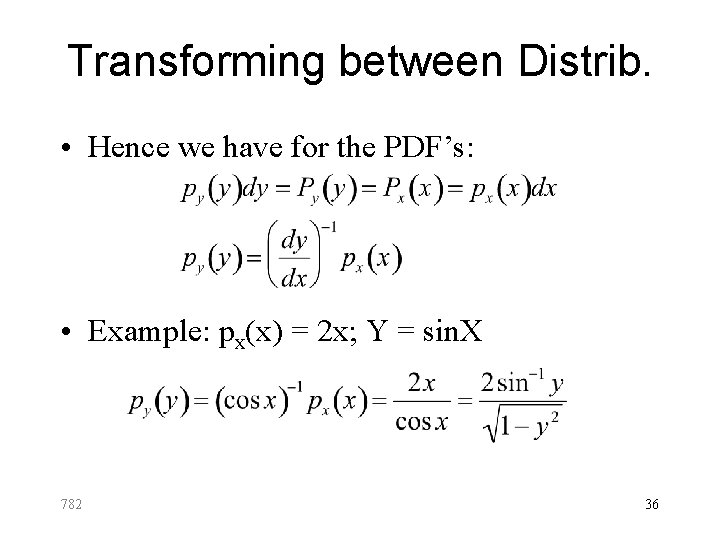
Transforming between Distrib. • Hence we have for the PDF’s: • Example: px(x) = 2 x; Y = sin. X 782 36

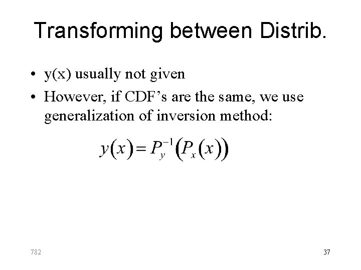
Transforming between Distrib. • y(x) usually not given • However, if CDF’s are the same, we use generalization of inversion method: 782 37

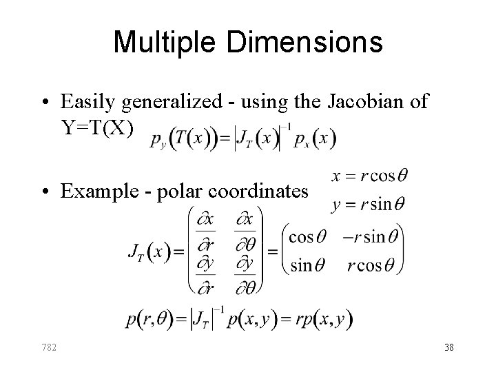
Multiple Dimensions • Easily generalized - using the Jacobian of Y=T(X) • Example - polar coordinates 782 38

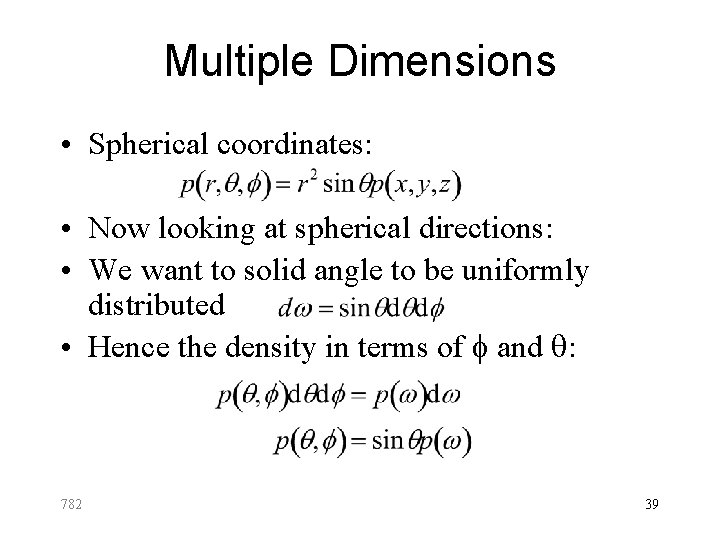
Multiple Dimensions • Spherical coordinates: • Now looking at spherical directions: • We want to solid angle to be uniformly distributed • Hence the density in terms of f and : 782 39

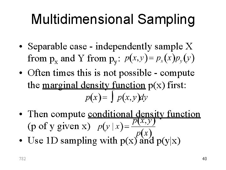
Multidimensional Sampling • Separable case - independently sample X from px and Y from py: • Often times this is not possible - compute the marginal density function p(x) first: • Then compute conditional density function (p of y given x) • Use 1 D sampling with p(x) and p(y|x) 782 40

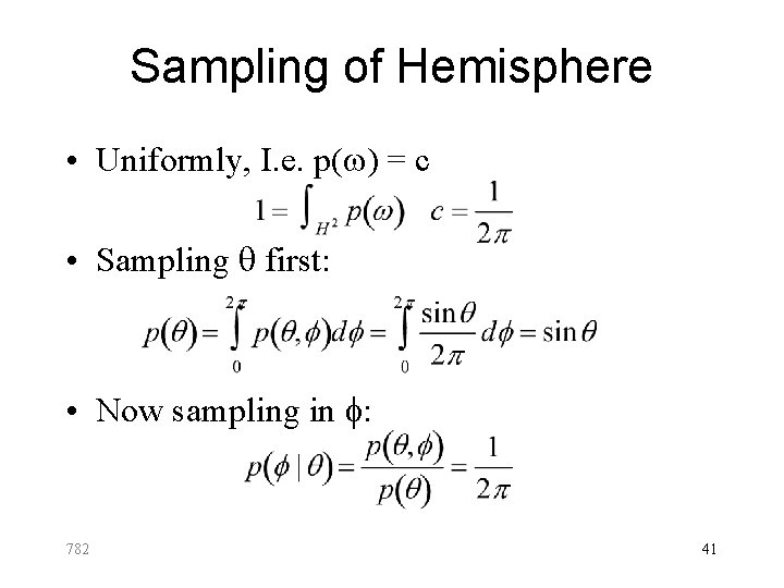
Sampling of Hemisphere • Uniformly, I. e. p(w) = c • Sampling first: • Now sampling in f: 782 41

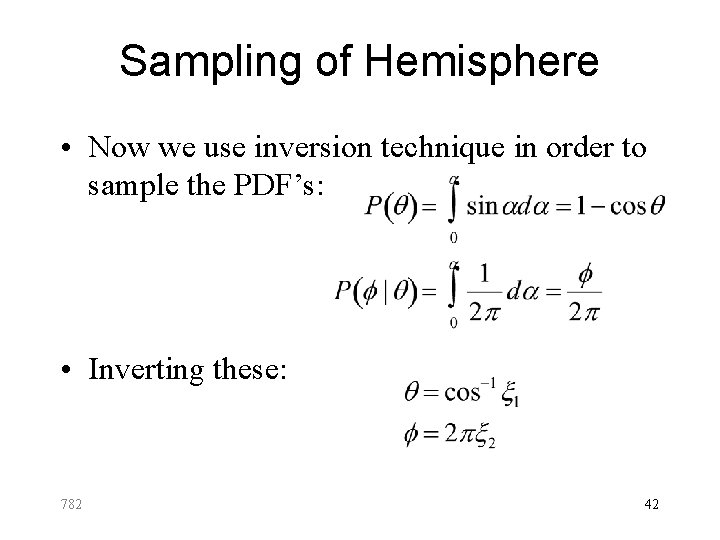
Sampling of Hemisphere • Now we use inversion technique in order to sample the PDF’s: • Inverting these: 782 42

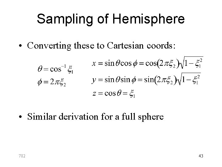
Sampling of Hemisphere • Converting these to Cartesian coords: • Similar derivation for a full sphere 782 43

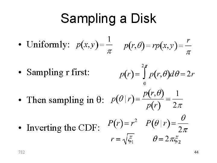
Sampling a Disk • Uniformly: • Sampling r first: • Then sampling in : • Inverting the CDF: 782 44

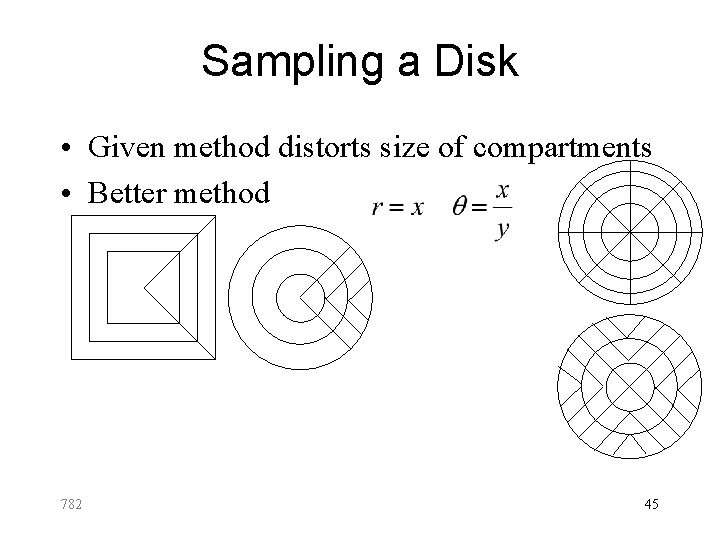
Sampling a Disk • Given method distorts size of compartments • Better method 782 45

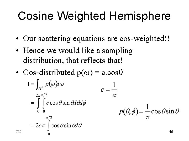
Cosine Weighted Hemisphere • Our scattering equations are cos-weighted!! • Hence we would like a sampling distribution, that reflects that! • Cos-distributed p(w) = c. cos 782 46

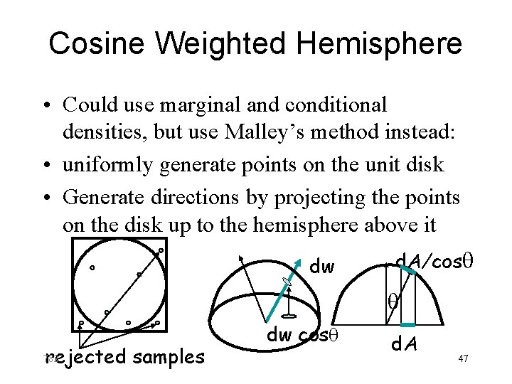
Cosine Weighted Hemisphere • Could use marginal and conditional densities, but use Malley’s method instead: • uniformly generate points on the unit disk • Generate directions by projecting the points on the disk up to the hemisphere above it dw d. A/cos rejected samples 782 dw cos d. A 47

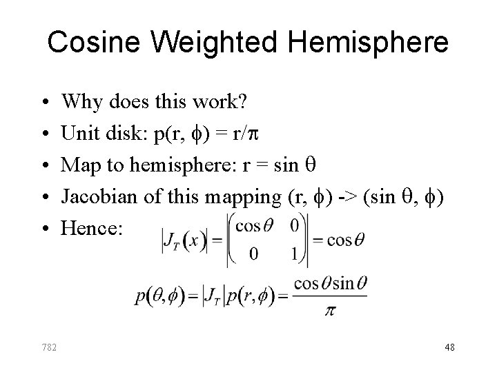
Cosine Weighted Hemisphere • • • 782 Why does this work? Unit disk: p(r, f) = r/p Map to hemisphere: r = sin Jacobian of this mapping (r, f) -> (sin , f) Hence: 48

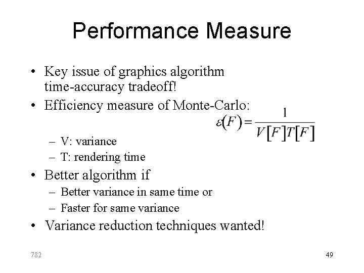
Performance Measure • Key issue of graphics algorithm time-accuracy tradeoff! • Efficiency measure of Monte-Carlo: – V: variance – T: rendering time • Better algorithm if – Better variance in same time or – Faster for same variance • Variance reduction techniques wanted! 782 49

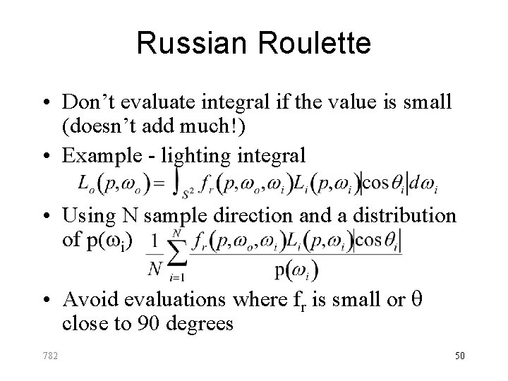
Russian Roulette • Don’t evaluate integral if the value is small (doesn’t add much!) • Example - lighting integral • Using N sample direction and a distribution of p(wi) • Avoid evaluations where fr is small or close to 90 degrees 782 50

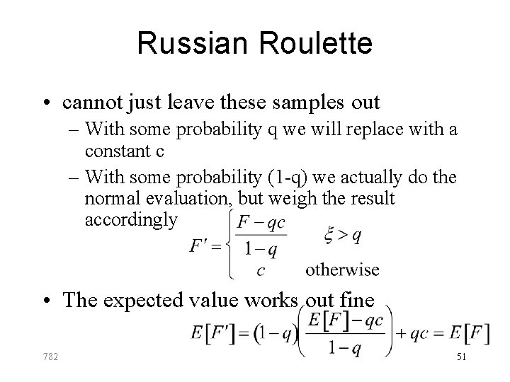
Russian Roulette • cannot just leave these samples out – With some probability q we will replace with a constant c – With some probability (1 -q) we actually do the normal evaluation, but weigh the result accordingly • The expected value works out fine 782 51

Russian Roulette • Increases variance • Improves speed dramatically • Don’t pick q to be high though!! 782 52

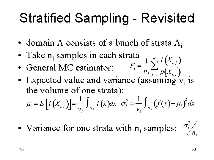
Stratified Sampling - Revisited • • domain L consists of a bunch of strata Li Take ni samples in each strata General MC estimator: Expected value and variance (assuming vi is the volume of one strata): • Variance for one strata with ni samples: 782 53

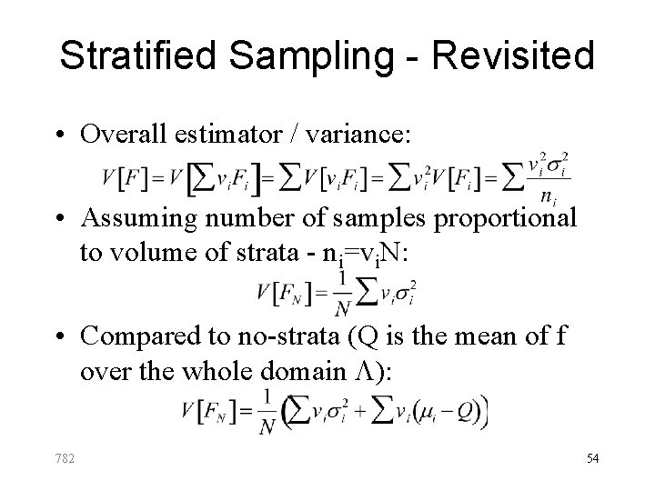
Stratified Sampling - Revisited • Overall estimator / variance: • Assuming number of samples proportional to volume of strata - ni=vi. N: • Compared to no-strata (Q is the mean of f over the whole domain L): 782 54

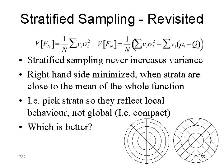
Stratified Sampling - Revisited • Stratified sampling never increases variance • Right hand side minimized, when strata are close to the mean of the whole function • I. e. pick strata so they reflect local behaviour, not global (I. e. compact) • Which is better? 782 55

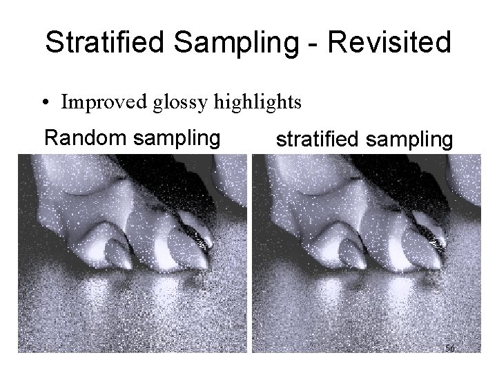
Stratified Sampling - Revisited • Improved glossy highlights Random sampling 782 stratified sampling 56

Stratified Sampling - Revisited • Curse of dimensionality • Alternative - Latin Hypercubes – Better variance than uniform random – Worse variance than stratified 782 57

Quasi Monte Carlo • Doesn’t use ‘real’ random numbers • Replaced by low-discrepancy sequences • Works well for many techniques including importance sampling • Doesn’t work as well for Russian Roulette and rejection sampling • Better convergence rate than regular MC 782 58

Bias • If b is zero - unbiased, otherwise biased • Example - pixel filtering • Unbiased MC estimator, with distribution p • Biased (regular) filtering: 782 59

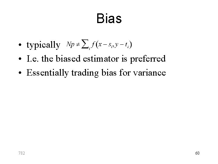
Bias • typically • I. e. the biased estimator is preferred • Essentially trading bias for variance 782 60

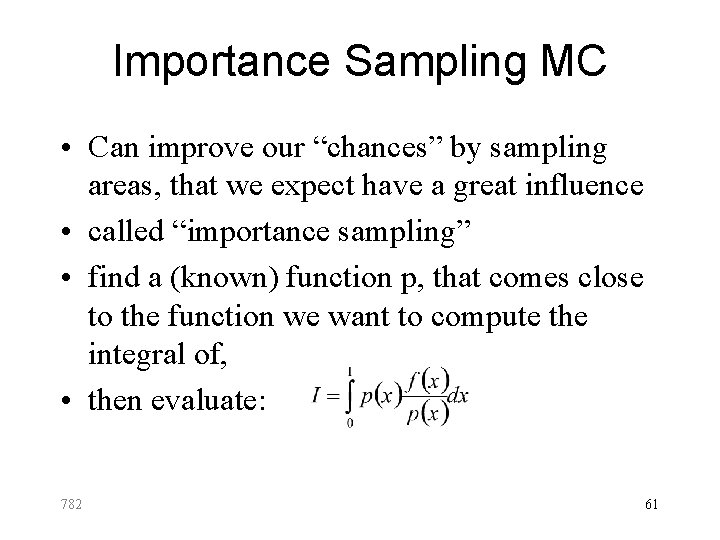
Importance Sampling MC • Can improve our “chances” by sampling areas, that we expect have a great influence • called “importance sampling” • find a (known) function p, that comes close to the function we want to compute the integral of, • then evaluate: 782 61

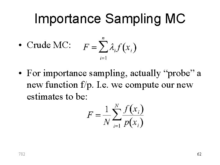
Importance Sampling MC • Crude MC: • For importance sampling, actually “probe” a new function f/p. I. e. we compute our new estimates to be: 782 62

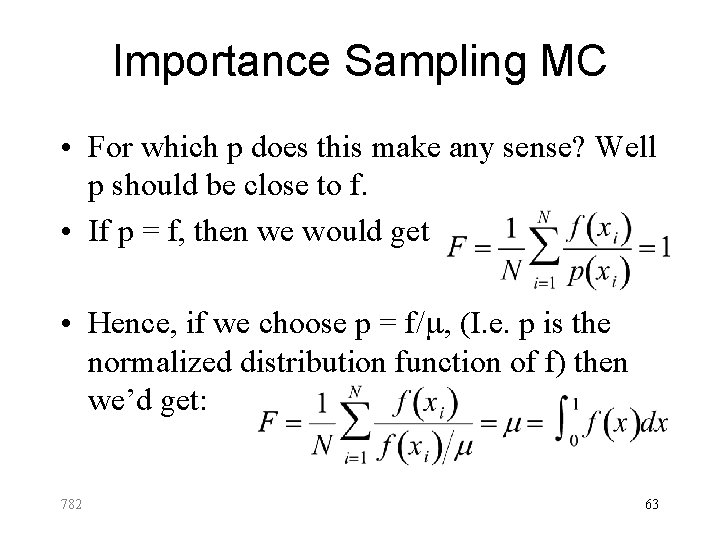
Importance Sampling MC • For which p does this make any sense? Well p should be close to f. • If p = f, then we would get • Hence, if we choose p = f/m, (I. e. p is the normalized distribution function of f) then we’d get: 782 63

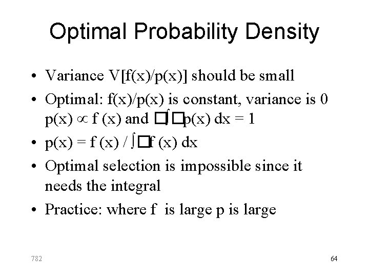
Optimal Probability Density • Variance V[f(x)/p(x)] should be small • Optimal: f(x)/p(x) is constant, variance is 0 p(x) f (x) and � �p(x) dx = 1 • p(x) = f (x) / �f (x) dx • Optimal selection is impossible since it needs the integral • Practice: where f is large p is large 782 64

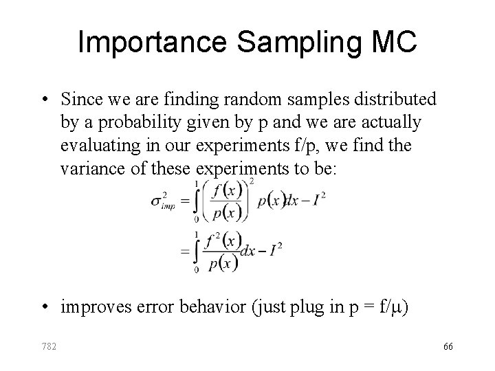
Importance Sampling MC • Since we are finding random samples distributed by a probability given by p and we are actually evaluating in our experiments f/p, we find the variance of these experiments to be: • improves error behavior (just plug in p = f/m) 782 66

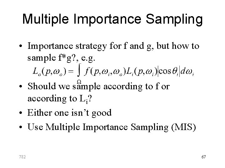
Multiple Importance Sampling • Importance strategy for f and g, but how to sample f*g? , e. g. • Should we sample according to f or according to Li? • Either one isn’t good • Use Multiple Importance Sampling (MIS) 782 67

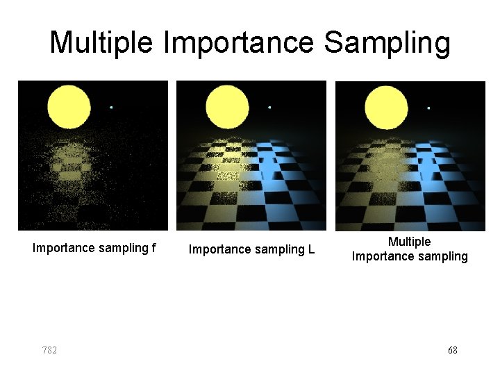
Multiple Importance Sampling Importance sampling f 782 Importance sampling L Multiple Importance sampling 68

Multiple Importance Sampling • In order to evaluate • Pick nf samples according to pf and ng samples according to pg • Use new MC estimator: • Balance heuristic vs. power heuristic: 782 69

MC for global illumination • We know the basics of MC • How to apply for global illumination? – How to apply to Bx. DF’s – How to apply to light source 782 70

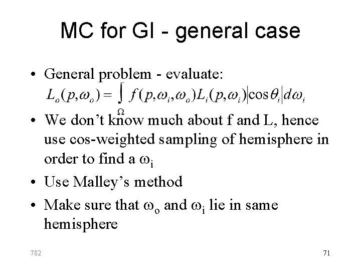
MC for GI - general case • General problem - evaluate: • We don’t know much about f and L, hence use cos-weighted sampling of hemisphere in order to find a wi • Use Malley’s method • Make sure that wo and wi lie in same hemisphere 782 71

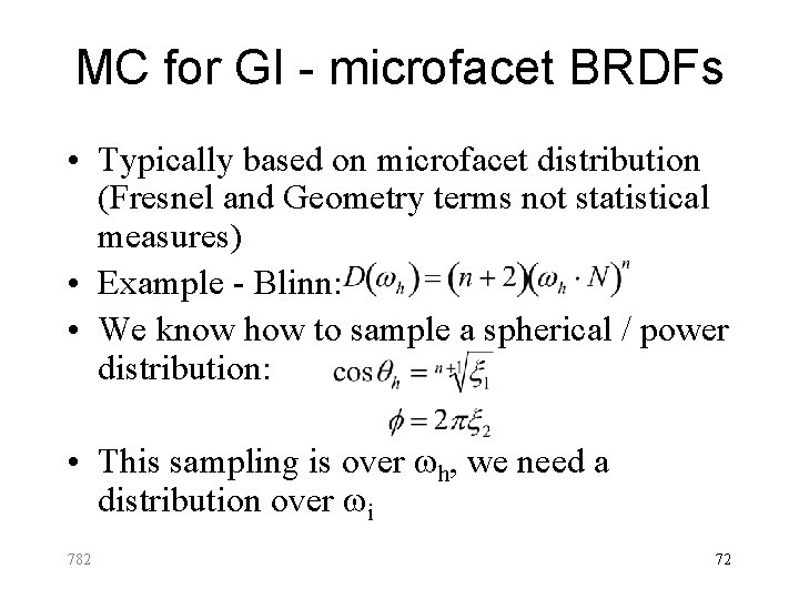
MC for GI - microfacet BRDFs • Typically based on microfacet distribution (Fresnel and Geometry terms not statistical measures) • Example - Blinn: • We know how to sample a spherical / power distribution: • This sampling is over wh, we need a distribution over wi 782 72

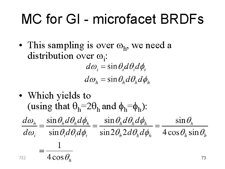
MC for GI - microfacet BRDFs • This sampling is over wh, we need a distribution over wi: • Which yields to (using that h=2 h and fh=fh): 782 73

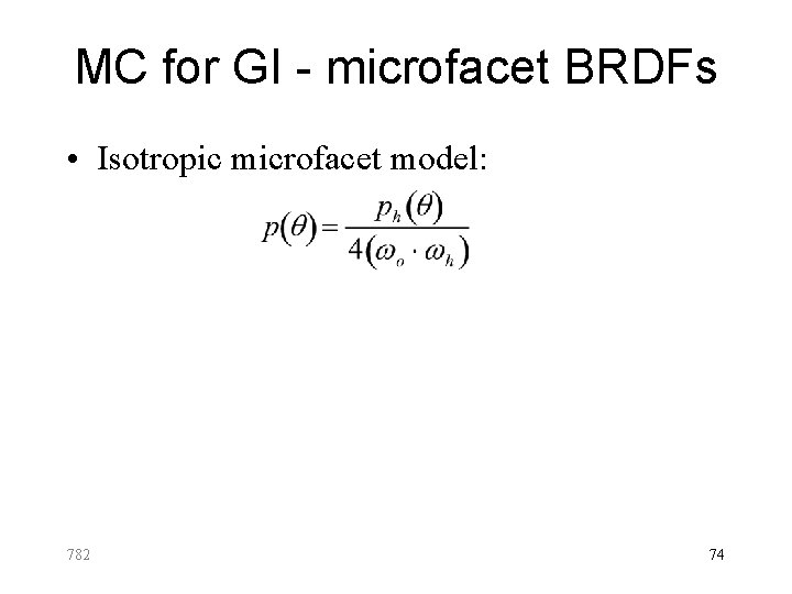
MC for GI - microfacet BRDFs • Isotropic microfacet model: 782 74

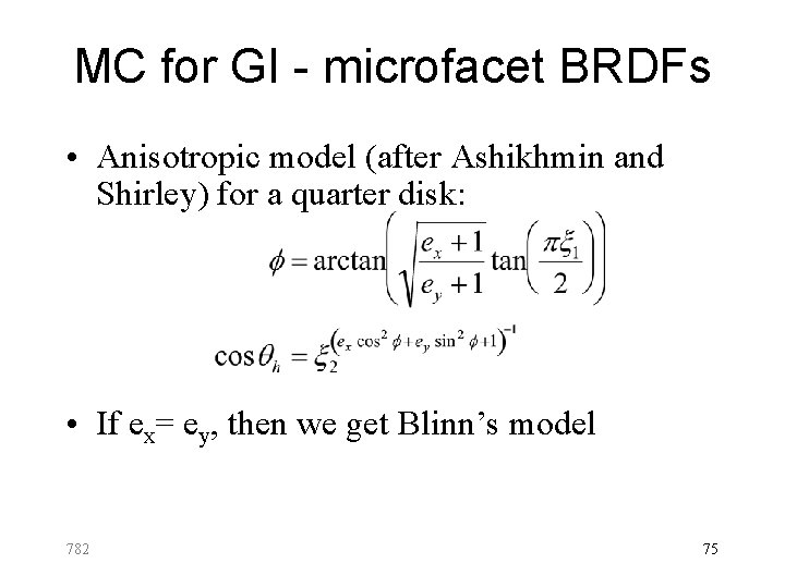
MC for GI - microfacet BRDFs • Anisotropic model (after Ashikhmin and Shirley) for a quarter disk: • If ex= ey, then we get Blinn’s model 782 75

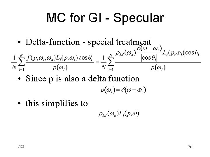
MC for GI - Specular • Delta-function - special treatment • Since p is also a delta function • this simplifies to 782 76

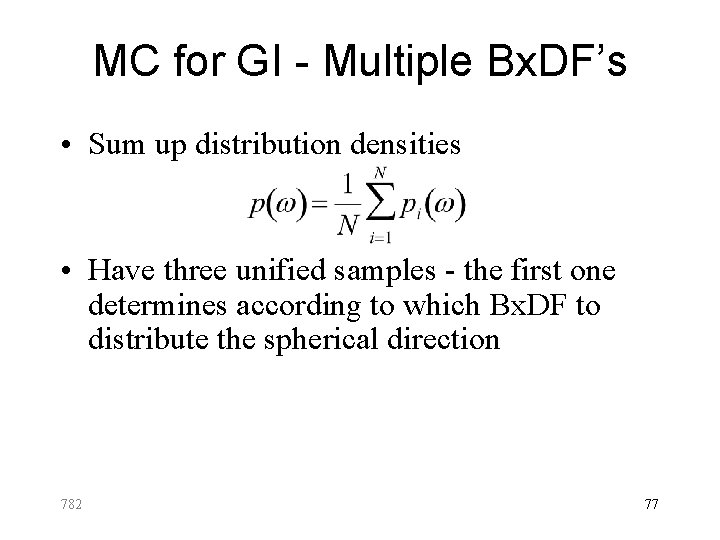
MC for GI - Multiple Bx. DF’s • Sum up distribution densities • Have three unified samples - the first one determines according to which Bx. DF to distribute the spherical direction 782 77

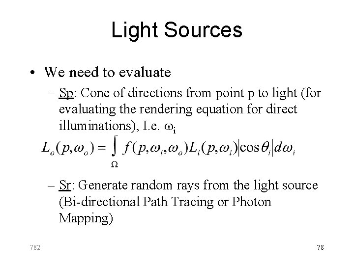
Light Sources • We need to evaluate – Sp: Cone of directions from point p to light (for evaluating the rendering equation for direct illuminations), I. e. wi – Sr: Generate random rays from the light source (Bi-directional Path Tracing or Photon Mapping) 782 78

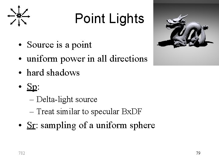
Point Lights • • Source is a point uniform power in all directions hard shadows Sp: – Delta-light source – Treat similar to specular Bx. DF • Sr: sampling of a uniform sphere 782 79

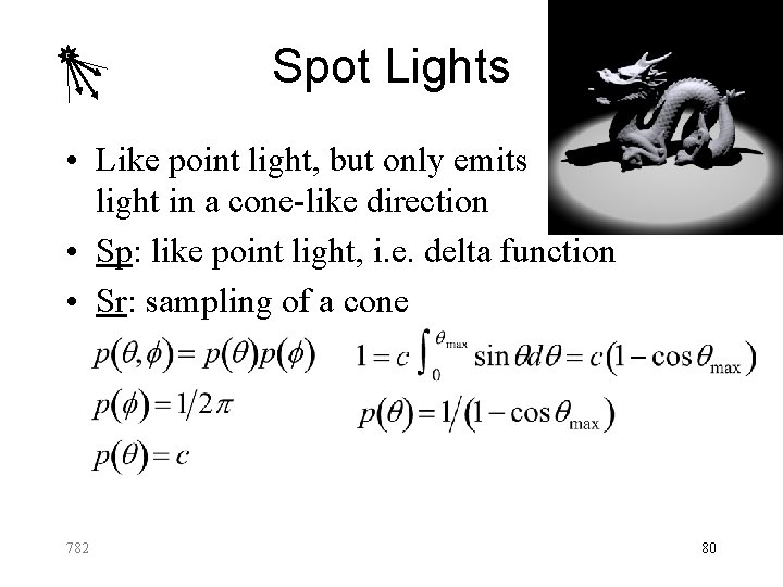
Spot Lights • Like point light, but only emits light in a cone-like direction • Sp: like point light, i. e. delta function • Sr: sampling of a cone 782 80

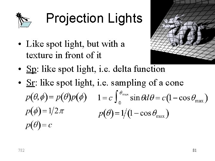
Projection Lights • Like spot light, but with a texture in front of it • Sp: like spot light, i. e. delta function • Sr: like spot light, i. e. sampling of a cone 782 81

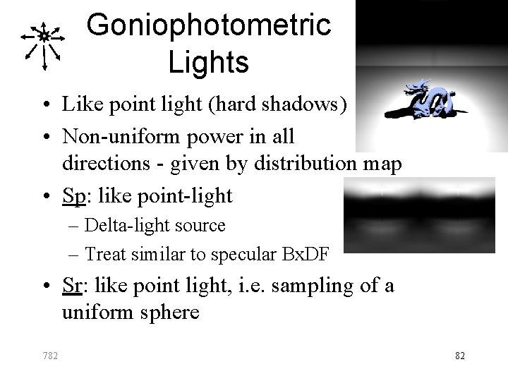
Goniophotometric Lights • Like point light (hard shadows) • Non-uniform power in all directions - given by distribution map • Sp: like point-light – Delta-light source – Treat similar to specular Bx. DF • Sr: like point light, i. e. sampling of a uniform sphere 782 82

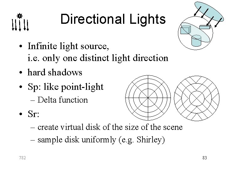
Directional Lights • Infinite light source, i. e. only one distinct light direction • hard shadows • Sp: like point-light – Delta function • Sr: – create virtual disk of the size of the scene – sample disk uniformly (e. g. Shirley) 782 83

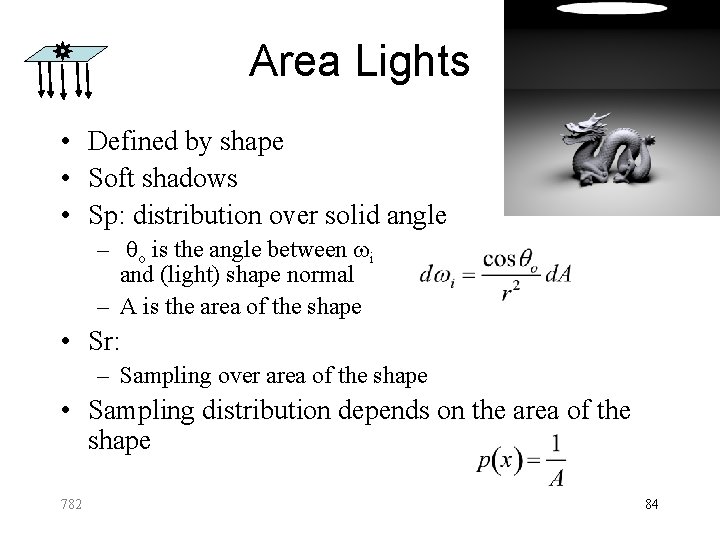
Area Lights • Defined by shape • Soft shadows • Sp: distribution over solid angle – o is the angle between wi and (light) shape normal – A is the area of the shape • Sr: – Sampling over area of the shape • Sampling distribution depends on the area of the shape 782 84

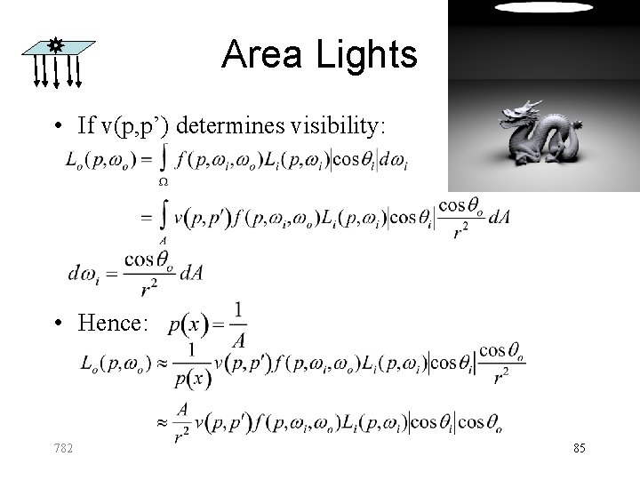
Area Lights • If v(p, p’) determines visibility: • Hence: 782 85

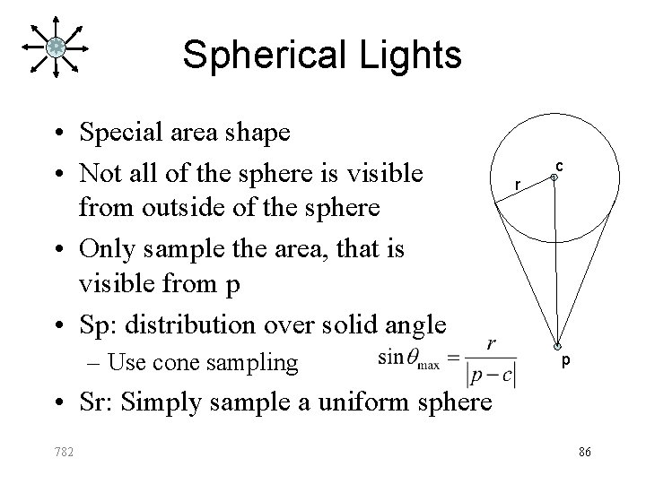
Spherical Lights • Special area shape • Not all of the sphere is visible from outside of the sphere • Only sample the area, that is visible from p • Sp: distribution over solid angle – Use cone sampling c r p • Sr: Simply sample a uniform sphere 782 86

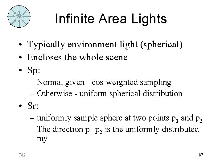
Infinite Area Lights • Typically environment light (spherical) • Encloses the whole scene • Sp: – Normal given - cos-weighted sampling – Otherwise - uniform spherical distribution • Sr: – uniformly sample sphere at two points p 1 and p 2 – The direction p 1 -p 2 is the uniformly distributed ray 782 87

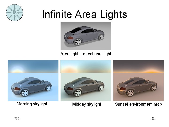
Infinite Area Lights Area light + directional light Morning skylight 782 Midday skylight Sunset environment map 88

Summary 782 89