THE NEUTRAL ATMOSPHERE Temperature and density structure Hydrogen

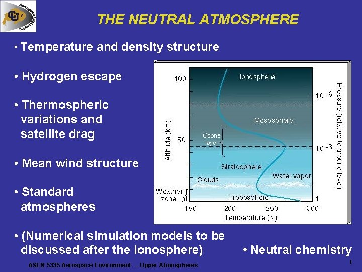
THE NEUTRAL ATMOSPHERE • Temperature and density structure • Hydrogen escape • Thermospheric variations and satellite drag • Mean wind structure • Standard atmospheres • (Numerical simulation models to be discussed after the ionosphere) ASEN 5335 Aerospace Environment -- Upper Atmospheres • Neutral chemistry 1

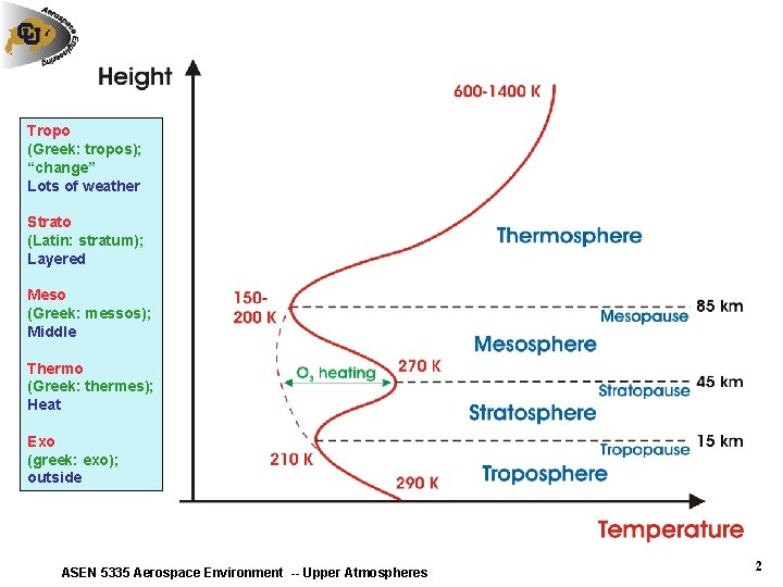
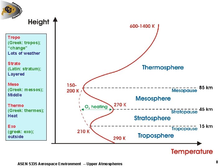
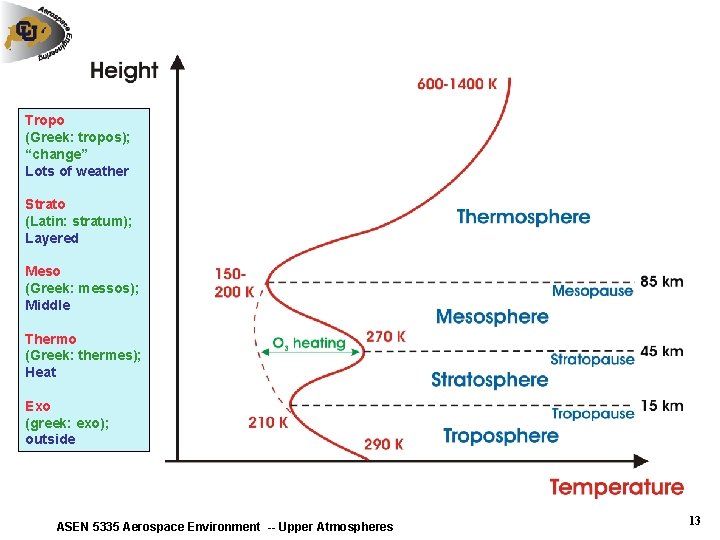
Tropo (Greek: tropos); “change” Lots of weather Strato (Latin: stratum); Layered Meso (Greek: messos); Middle Thermo (Greek: thermes); Heat Exo (greek: exo); outside ASEN 5335 Aerospace Environment -- Upper Atmospheres 2

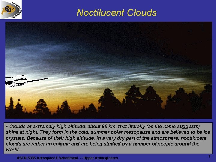
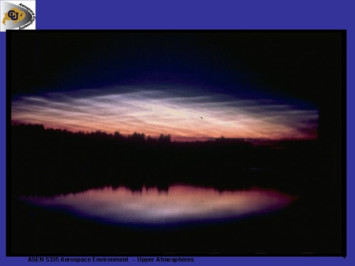
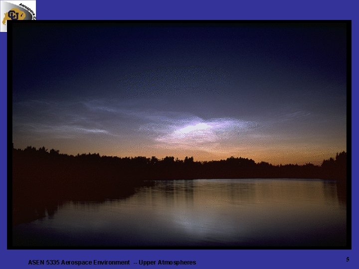
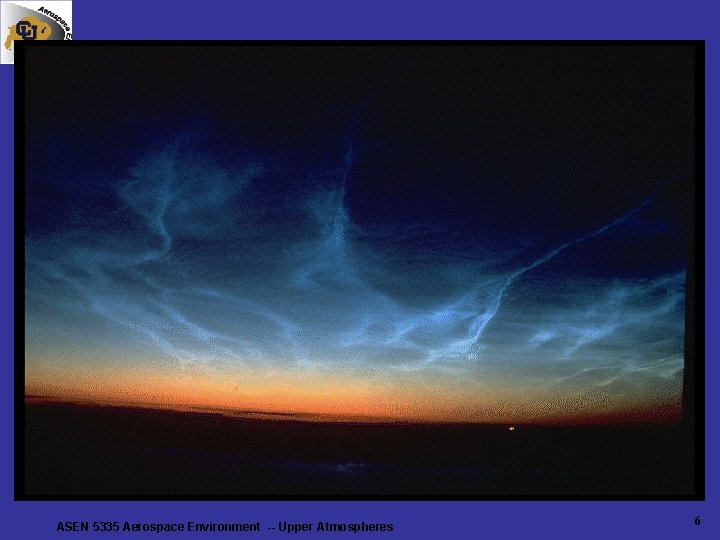
Noctilucent Clouds § Clouds at extremely high altitude, about 85 km, that literally (as the name suggests) shine at night. They form in the cold, summer polar mesopause and are believed to be ice crystals. Because of their high altitude, in a very dry part of the atmosphere, noctilucent clouds are rather an enigma and are being studied by a number of people around the world. ASEN 5335 Aerospace Environment -- Upper Atmospheres 3

ASEN 5335 Aerospace Environment -- Upper Atmospheres 4

ASEN 5335 Aerospace Environment -- Upper Atmospheres 5

ASEN 5335 Aerospace Environment -- Upper Atmospheres 6

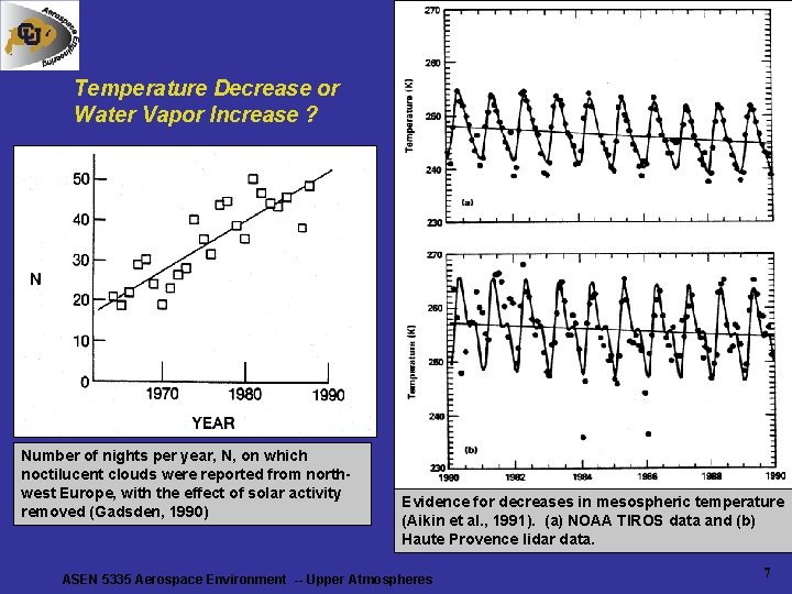
Temperature Decrease or Water Vapor Increase ? Number of nights per year, N, on which noctilucent clouds were reported from northwest Europe, with the effect of solar activity removed (Gadsden, 1990) Evidence for decreases in mesospheric temperature (Aikin et al. , 1991). (a) NOAA TIROS data and (b) Haute Provence lidar data. ASEN 5335 Aerospace Environment -- Upper Atmospheres 7

Tropo (Greek: tropos); “change” Lots of weather Strato (Latin: stratum); Layered Meso (Greek: messos); Middle Thermo (Greek: thermes); Heat Exo (greek: exo); outside ASEN 5335 Aerospace Environment -- Upper Atmospheres 8

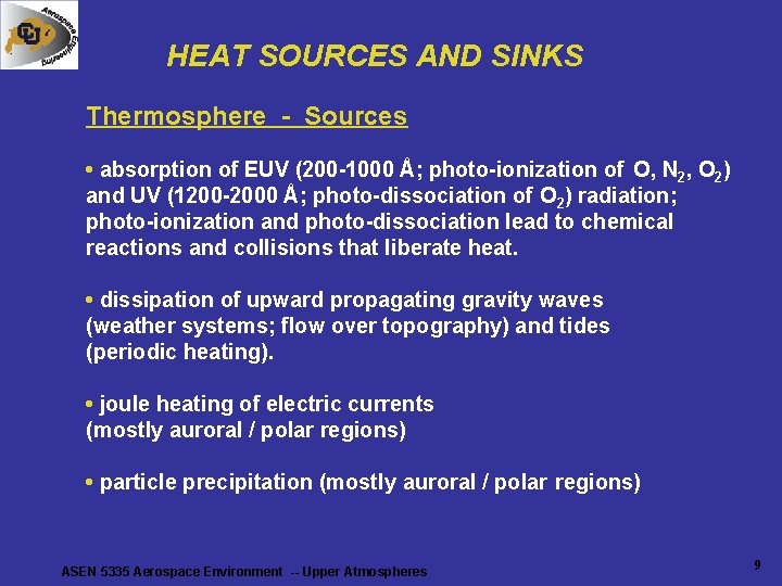
HEAT SOURCES AND SINKS Thermosphere - Sources • absorption of EUV (200 -1000 Å; photo-ionization of O, N 2, O 2) and UV (1200 -2000 Å; photo-dissociation of O 2) radiation; photo-ionization and photo-dissociation lead to chemical reactions and collisions that liberate heat. • dissipation of upward propagating gravity waves (weather systems; flow over topography) and tides (periodic heating). • joule heating of electric currents (mostly auroral / polar regions) • particle precipitation (mostly auroral / polar regions) ASEN 5335 Aerospace Environment -- Upper Atmospheres 9

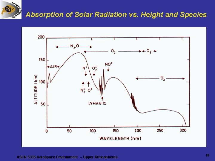
Absorption of Solar Radiation vs. Height and Species ASEN 5335 Aerospace Environment -- Upper Atmospheres 10

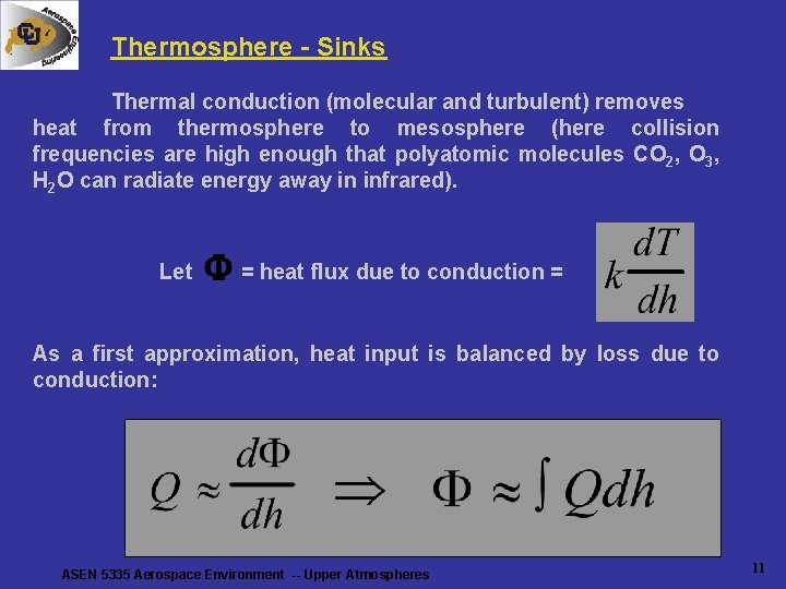
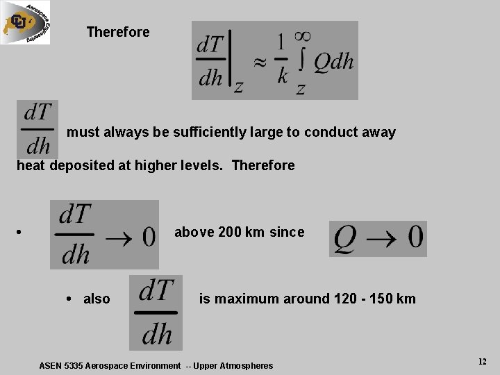
Thermosphere - Sinks Thermal conduction (molecular and turbulent) removes heat from thermosphere to mesosphere (here collision frequencies are high enough that polyatomic molecules CO 2, O 3, H 2 O can radiate energy away in infrared). Let = heat flux due to conduction = As a first approximation, heat input is balanced by loss due to conduction: ASEN 5335 Aerospace Environment -- Upper Atmospheres 11

Therefore must always be sufficiently large to conduct away heat deposited at higher levels. Therefore • above 200 km since • also is maximum around 120 - 150 km ASEN 5335 Aerospace Environment -- Upper Atmospheres 12

Tropo (Greek: tropos); “change” Lots of weather Strato (Latin: stratum); Layered Meso (Greek: messos); Middle Thermo (Greek: thermes); Heat Exo (greek: exo); outside ASEN 5335 Aerospace Environment -- Upper Atmospheres 13

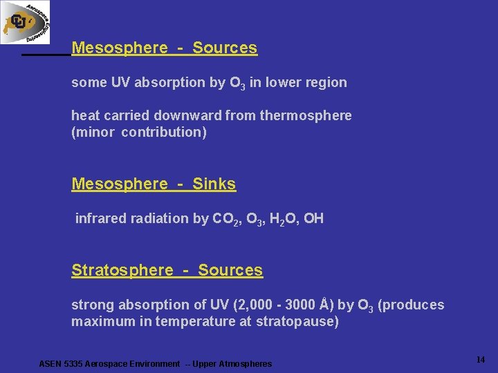
Mesosphere - Sources some UV absorption by O 3 in lower region heat carried downward from thermosphere (minor contribution) Mesosphere - Sinks infrared radiation by CO 2, O 3, H 2 O, OH Stratosphere - Sources strong absorption of UV (2, 000 - 3000 Å) by O 3 (produces maximum in temperature at stratopause) ASEN 5335 Aerospace Environment -- Upper Atmospheres 14

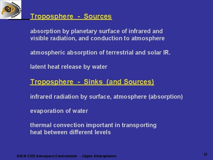
Troposphere - Sources absorption by planetary surface of infrared and visible radiation, and conduction to atmosphere atmospheric absorption of terrestrial and solar IR. latent heat release by water Troposphere - Sinks (and Sources) infrared radiation by surface, atmosphere (absorption) evaporation of water thermal convection important in transporting heat between different levels ASEN 5335 Aerospace Environment -- Upper Atmospheres 15

Aerospace Environment ASEN-5335 • Instructor: Prof. Xinlin Li (pronounce: Shinlyn Lee) • Contact info: e-mail: lix@lasp. colorado. edu (preferred) phone: 2 -3514, or 5 -0523, fax: 2 -6444, website: http: //lasp. colorado. edu/~lix • Instructor’s office hours: 9 -11 am at ECOT 534 • TA’s office hours: 3: 15 -5: 15 pm Wed at ECAE 166. E-mail: Christopher. Hood@colorado. edu • • READ classnotes and Chapter 6 HW 6 due today Quiz-7 on 4/29 HW 7 due 5/1 ASEN 5335 Aerospace Environment -- Upper Atmospheres 16

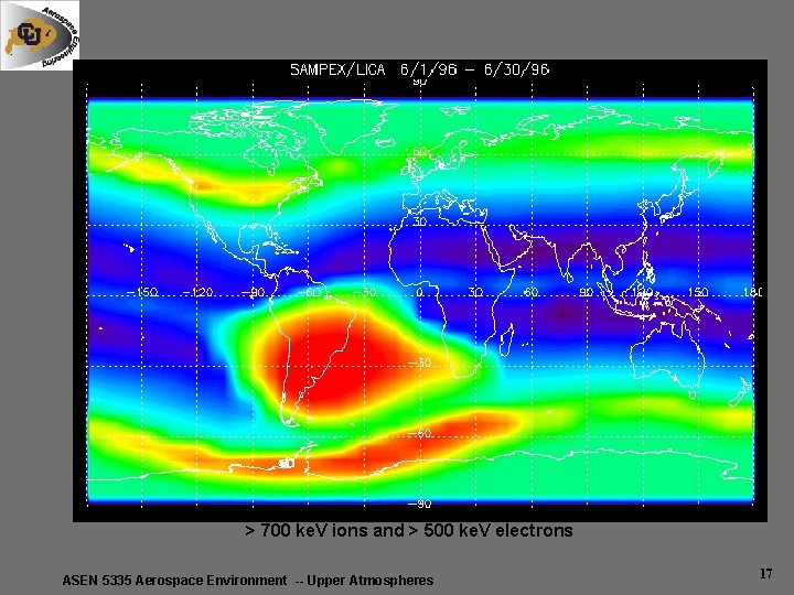
> 700 ke. V ions and > 500 ke. V electrons ASEN 5335 Aerospace Environment -- Upper Atmospheres 17

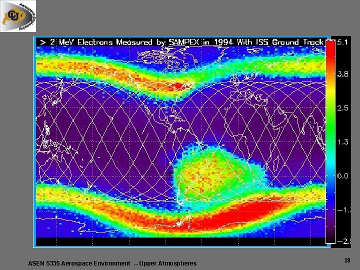
ASEN 5335 Aerospace Environment -- Upper Atmospheres 18

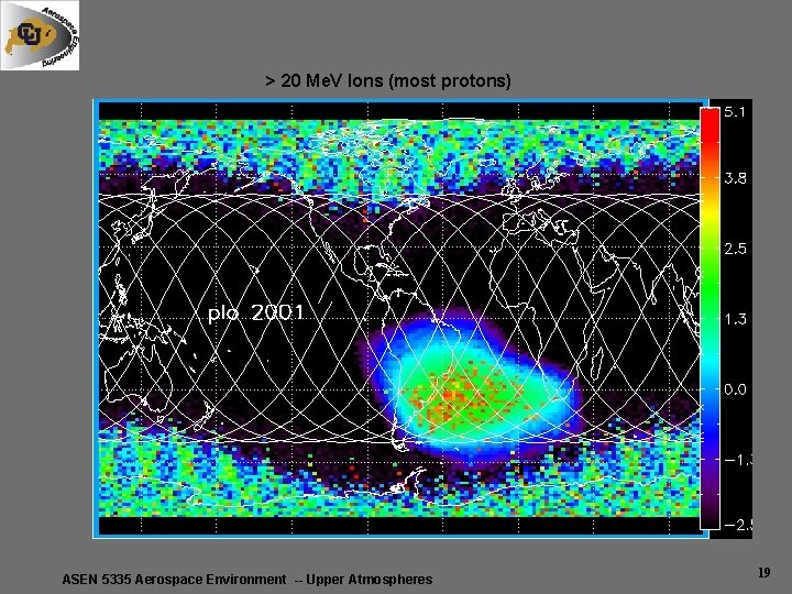
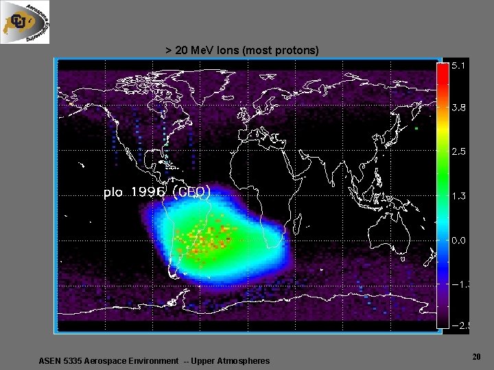
> 20 Me. V Ions (most protons) ASEN 5335 Aerospace Environment -- Upper Atmospheres 19

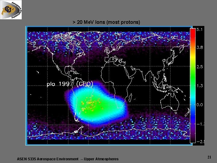
> 20 Me. V Ions (most protons) ASEN 5335 Aerospace Environment -- Upper Atmospheres 20

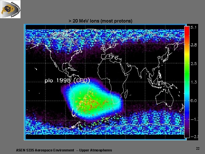
> 20 Me. V Ions (most protons) ASEN 5335 Aerospace Environment -- Upper Atmospheres 21

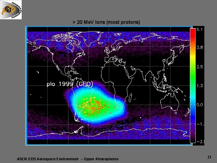
> 20 Me. V Ions (most protons) ASEN 5335 Aerospace Environment -- Upper Atmospheres 22

> 20 Me. V Ions (most protons) ASEN 5335 Aerospace Environment -- Upper Atmospheres 23

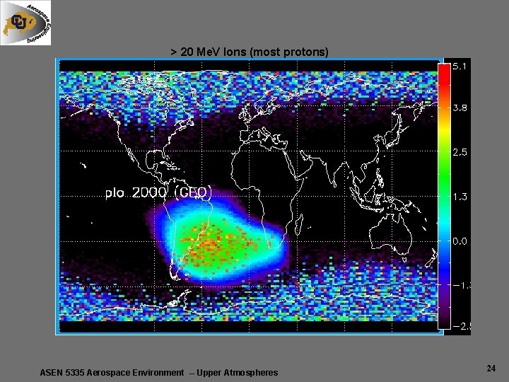
> 20 Me. V Ions (most protons) ASEN 5335 Aerospace Environment -- Upper Atmospheres 24

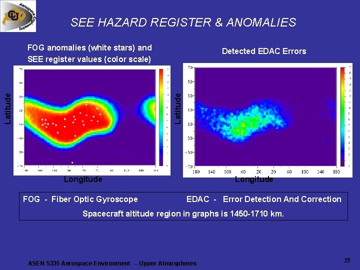
SEE HAZARD REGISTER & ANOMALIES FOG anomalies (white stars) and SEE register values (color scale) Latitude Detected EDAC Errors Longitude FOG - Fiber Optic Gyroscope Longitude EDAC - Error Detection And Correction Spacecraft altitude region in graphs is 1450 -1710 km. ASEN 5335 Aerospace Environment -- Upper Atmospheres 25

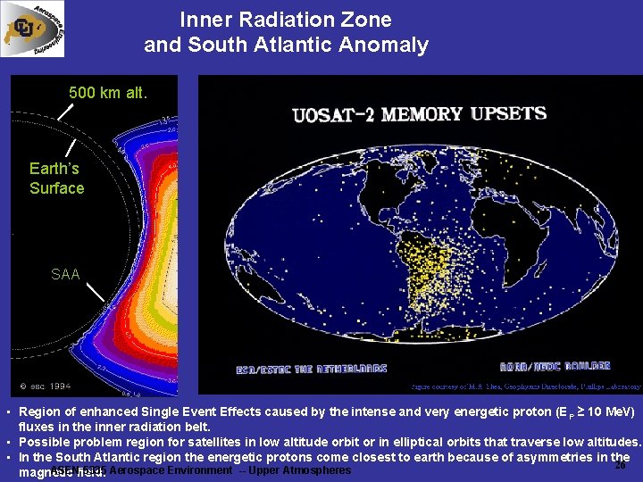
Inner Radiation Zone and South Atlantic Anomaly 500 km alt. Earth’s Surface SAA • Region of enhanced Single Event Effects caused by the intense and very energetic proton (E P ≥ 10 Me. V) fluxes in the inner radiation belt. • Possible problem region for satellites in low altitude orbit or in elliptical orbits that traverse low altitudes. • In the South Atlantic region the energetic protons come closest to earth because of asymmetries in the 26 ASENfield. 5335 Aerospace Environment -- Upper Atmospheres magnetic

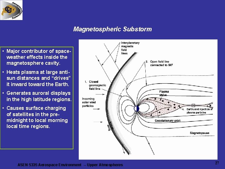
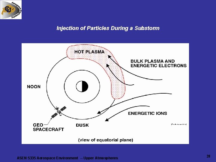
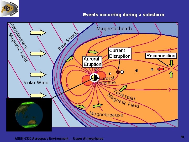
Magnetospheric Substorm • Major contributor of spaceweather effects inside the magnetosphere cavity. • Heats plasma at large antisun distances and “drives” it inward toward the Earth. • Generates auroral displays in the high latitude regions. • Causes surface charging of satellites in the premidnight to local morning local time regions. ASEN 5335 Aerospace Environment -- Upper Atmospheres 27

Injection of Particles During a Substorm (The Aerospace Corp. ) ASEN 5335 Aerospace Environment -- Upper Atmospheres 28

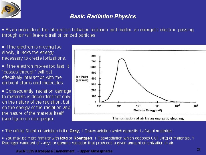
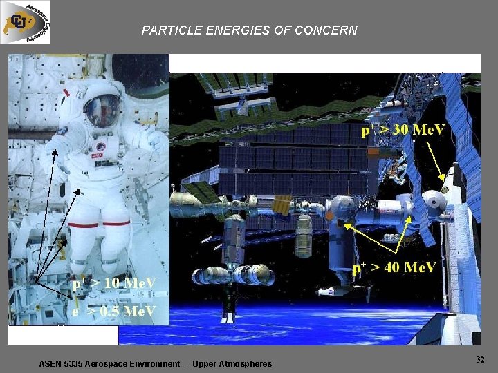
Basic Radiation Physics § As an example of the interaction between radiation and matter, an energetic electron passing through air will leave a trail of ionized particles. § If the electron is moving too slowly, it lacks the energy necessary to create ionizations. § If the electron moves too fast, it “passes through” without effectively interaction with the ambient atoms and molecules. § Consequently, radiation damage to materials is dependent not only on the nature of the radiation, but on the energy of the radiation and the nature of the material itself (see figure on next page). § The official SI unit of radiation is the Gray, 1 Gray=radiation which deposits 1 J/Kg of materials. § You may be more familiar with Rad or Roentgen: 1 Rad=radiation which deposits 0. 01 J/Kg of materials. 1 Roentgen=amount of x-rays or gamma radiation that produces a given amount of ionization in air. ASEN 5335 Aerospace Environment -- Upper Atmospheres 29

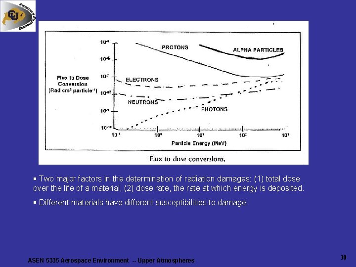
§ Two major factors in the determination of radiation damages: (1) total dose over the life of a material, (2) dose rate, the rate at which energy is deposited. § Different materials have different susceptibilities to damage: ASEN 5335 Aerospace Environment -- Upper Atmospheres 30

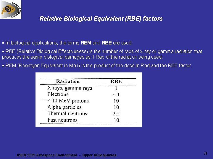
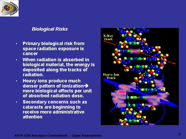
Relative Biological Equivalent (RBE) factors § In biological applications, the terms REM and RBE are used. § RBE (Relative Biological Effectiveness) is the number of rads of x-ray or gamma radiation that produces the same biological damages as 1 Rad of the radiation being used. § REM (Roentgen Equivalent in Man) is the product of the dose in Rad and the RBE factor. ASEN 5335 Aerospace Environment -- Upper Atmospheres 31

PARTICLE ENERGIES OF CONCERN ASEN 5335 Aerospace Environment -- Upper Atmospheres 32

Biological Risks • • Primary biological risk from space radiation exposure is cancer When radiation is absorbed in biological material, the energy is deposited along the tracks of radiation. Heavy ions produce much denser pattern of ionization more biological effects per unit of absorbed radiation dose. Secondary concerns such as cataracts are beginning to receive more administrative attention ASEN 5335 Aerospace Environment -- Upper Atmospheres 33

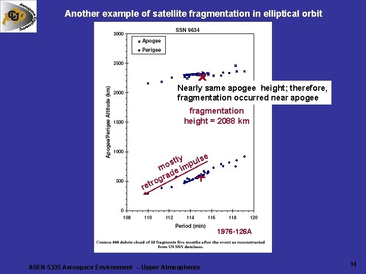
Another example of satellite fragmentation in elliptical orbit Nearly same apogee height; therefore, fragmentation occurred near apogee fragmentation height = 2088 km tly pulse s mo e im rad g ro ret + 1976 -126 A ASEN 5335 Aerospace Environment -- Upper Atmospheres 34

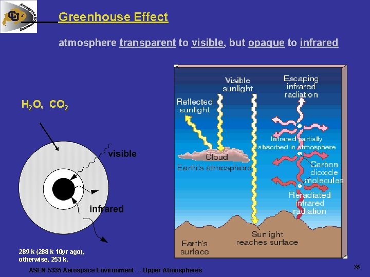
Greenhouse Effect atmosphere transparent to visible, but opaque to infrared H 2 O, CO 2 289 k (288 k 10 yr ago), otherwise, 253 k. ASEN 5335 Aerospace Environment -- Upper Atmospheres 35

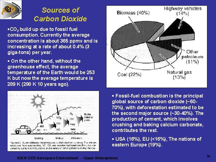
Sources of Carbon Dioxide §CO 2 build up due to fossil fuel consumption. Currently the average concentration is about 365 ppmv and is increasing at a rate of about 0. 4% (3 giga-tons) per year. § On the other hand, without the greenhouse effect, the average temperature of the Earth would be 253 K but now the average temperature is 289 K (288 K 10 years ago). § Fossil-fuel combustion is the principal global source of carbon dioxide (~6070%), with deforestation estimated to be the second major source (~30 -40%). The production of cement, which involves crushing and baking calcium carbonate, contributes the rest. § USA (16%), EU (<16%), The nations of eastern Europe (19%). ASEN 5335 Aerospace Environment -- Upper Atmospheres 36

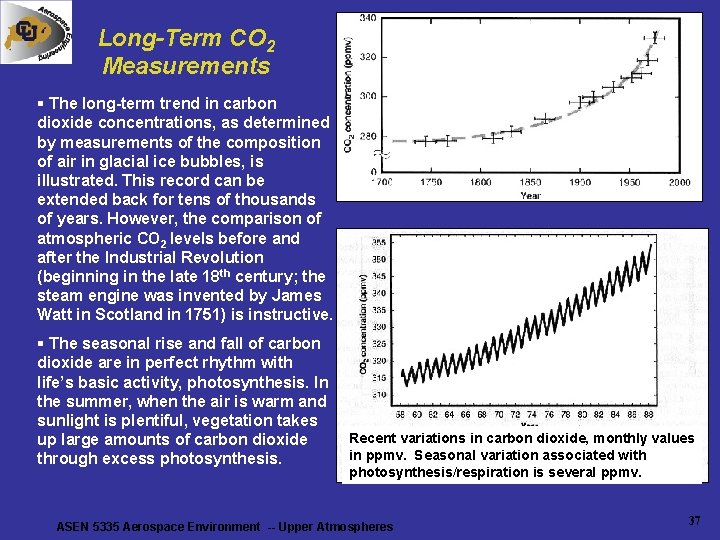
Long-Term CO 2 Measurements § The long-term trend in carbon dioxide concentrations, as determined by measurements of the composition of air in glacial ice bubbles, is illustrated. This record can be extended back for tens of thousands of years. However, the comparison of atmospheric CO 2 levels before and after the Industrial Revolution (beginning in the late 18 th century; the steam engine was invented by James Watt in Scotland in 1751) is instructive. § The seasonal rise and fall of carbon dioxide are in perfect rhythm with life’s basic activity, photosynthesis. In the summer, when the air is warm and sunlight is plentiful, vegetation takes up large amounts of carbon dioxide through excess photosynthesis. Recent variations in carbon dioxide, monthly values in ppmv. Seasonal variation associated with photosynthesis/respiration is several ppmv. ASEN 5335 Aerospace Environment -- Upper Atmospheres 37

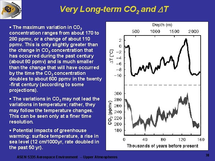
Very Long-term CO 2 and T § The maximum variation in CO 2 concentration ranges from about 170 to 280 ppmv, or a change of about 110 ppmv. This is only slightly greater than the change in CO 2 concentration that has occurred during the past century (about 80 ppmv) and is much smaller than the change that will have occurred by the time the CO 2 concentration doubles to about 600 ppmv in the twenty -first century (according to some projections). § The variations in CO 2 may not lead the variations in temperature; rather, they may follow the temperature changes. This can be seen only at a finer time resolution. § Potential impacts of greenhouse warming: surface temperature, a rise in sea level (12 cm/1000 yr, rate doubled in the past 50 yr). ASEN 5335 Aerospace Environment -- Upper Atmospheres 38

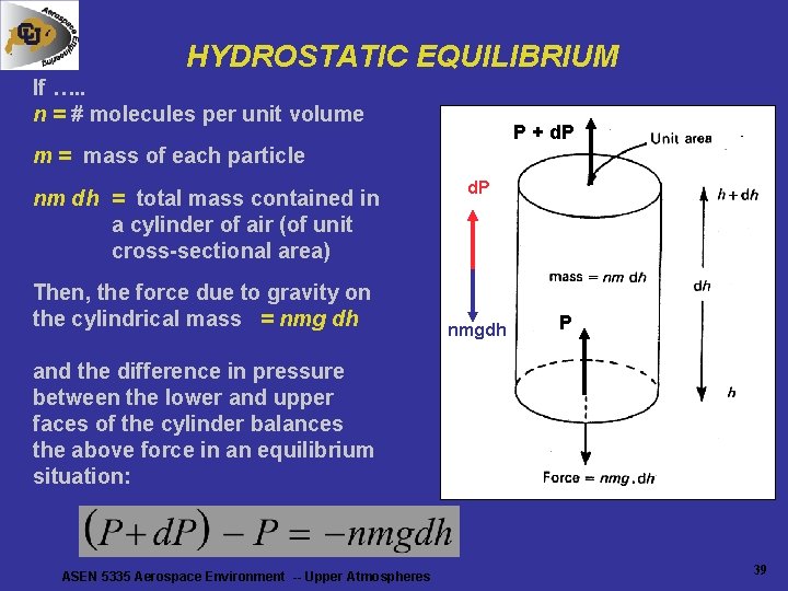
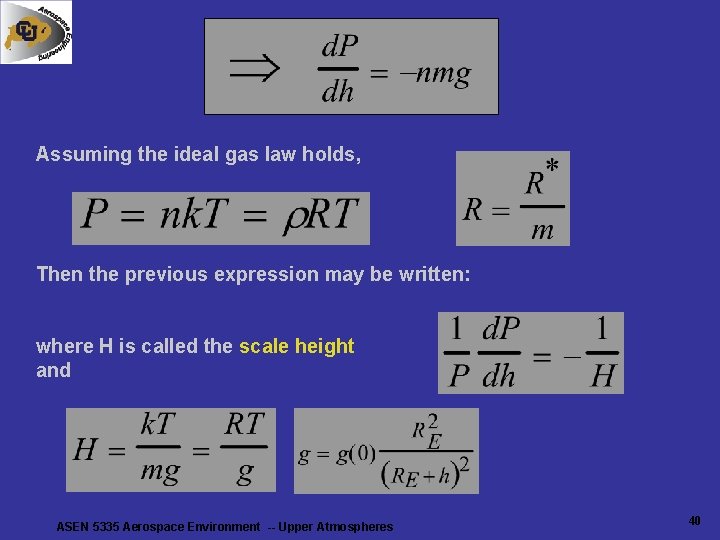
HYDROSTATIC EQUILIBRIUM If …. . n = # molecules per unit volume P + d. P m = mass of each particle nm dh = total mass contained in a cylinder of air (of unit cross-sectional area) Then, the force due to gravity on the cylindrical mass = nmg dh d. P nmgdh P and the difference in pressure between the lower and upper faces of the cylinder balances the above force in an equilibrium situation: ASEN 5335 Aerospace Environment -- Upper Atmospheres 39

Assuming the ideal gas law holds, Then the previous expression may be written: where H is called the scale height and ASEN 5335 Aerospace Environment -- Upper Atmospheres 40

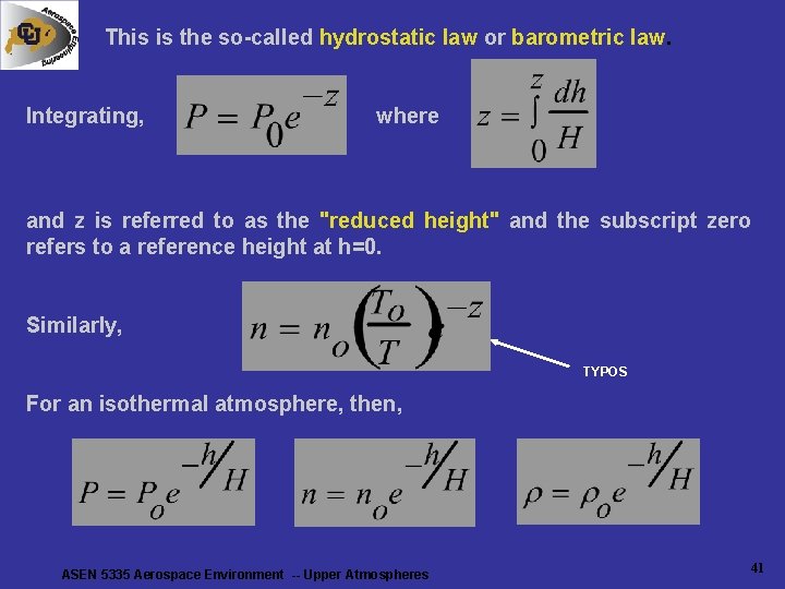
This is the so-called hydrostatic law or barometric law. Integrating, where and z is referred to as the "reduced height" and the subscript zero refers to a reference height at h=0. Similarly, TYPOS For an isothermal atmosphere, then, ASEN 5335 Aerospace Environment -- Upper Atmospheres 41

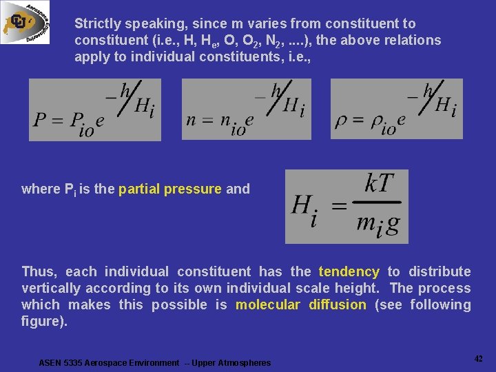
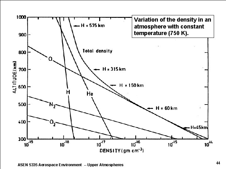
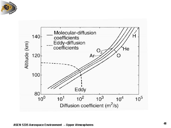
Strictly speaking, since m varies from constituent to constituent (i. e. , H, He, O, O 2, N 2, . . ), the above relations apply to individual constituents, i. e. , where Pi is the partial pressure and Thus, each individual constituent has the tendency to distribute vertically according to its own individual scale height. The process which makes this possible is molecular diffusion (see following figure). ASEN 5335 Aerospace Environment -- Upper Atmospheres 42

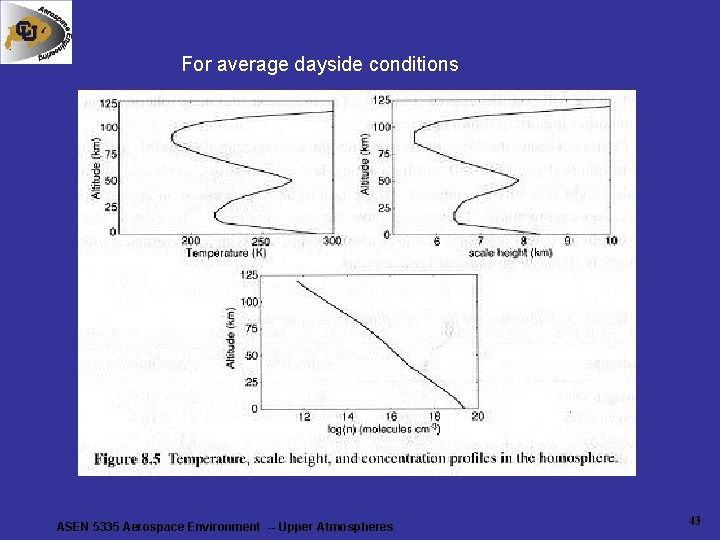
For average dayside conditions ASEN 5335 Aerospace Environment -- Upper Atmospheres 43

Variation of the density in an atmosphere with constant temperature (750 K). ASEN 5335 Aerospace Environment -- Upper Atmospheres 44

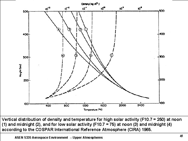
Vertical distribution of density and temperature for high solar activity (F 10. 7 = 250) at noon (1) and midnight (2), and for low solar activity (F 10. 7 = 75) at noon (3) and midnight (4) according to the COSPAR International Reference Atmosphere (CIRA) 1965. ASEN 5335 Aerospace Environment -- Upper Atmospheres 45

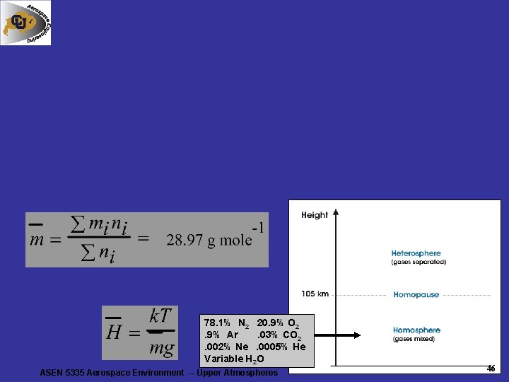
78. 1% N 2 20. 9% O 2. 9% Ar. 03% CO 2. 002% Ne. 0005% He Variable H 2 O ASEN 5335 Aerospace Environment -- Upper Atmospheres 46

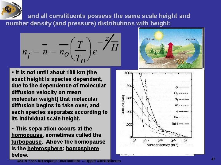
and all constituents possess the same scale height and number density (and pressure) distributions with height: § It is not until about 100 km (the exact height is species dependent, due to the dependence of molecular diffusion velocity on mean molecular weight) that molecular diffusion begins to take over, and each species separates according to its individual scale height. § This separation occurs at the homopause, sometimes called the turbopause. Above the homopause is the heterosphere; homosphere below. ASEN 5335 Aerospace Environment -- Upper Atmospheres 47

ASEN 5335 Aerospace Environment -- Upper Atmospheres 48

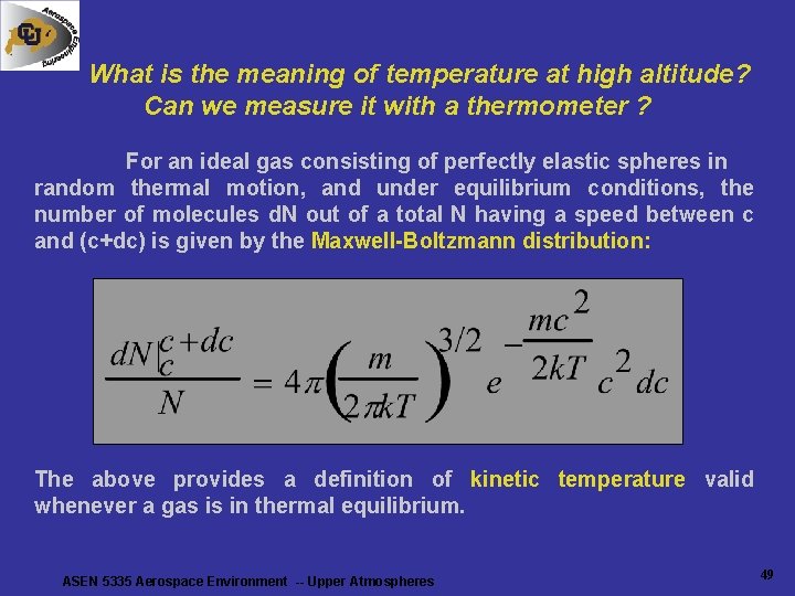
What is the meaning of temperature at high altitude? Can we measure it with a thermometer ? For an ideal gas consisting of perfectly elastic spheres in random thermal motion, and under equilibrium conditions, the number of molecules d. N out of a total N having a speed between c and (c+dc) is given by the Maxwell-Boltzmann distribution: The above provides a definition of kinetic temperature valid whenever a gas is in thermal equilibrium. ASEN 5335 Aerospace Environment -- Upper Atmospheres 49

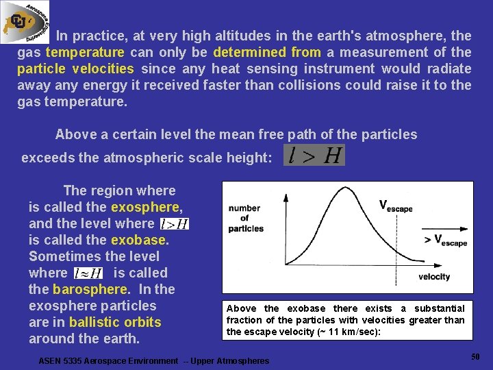
In practice, at very high altitudes in the earth's atmosphere, the gas temperature can only be determined from a measurement of the particle velocities since any heat sensing instrument would radiate away any energy it received faster than collisions could raise it to the gas temperature. Above a certain level the mean free path of the particles exceeds the atmospheric scale height: The region where is called the exosphere, and the level where is called the exobase. Sometimes the level where is called the barosphere. In the exosphere particles are in ballistic orbits around the earth. Above the exobase there exists a substantial fraction of the particles with velocities greater than the escape velocity (~ 11 km/sec): ASEN 5335 Aerospace Environment -- Upper Atmospheres 50

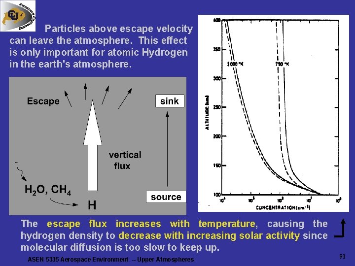
Particles above escape velocity can leave the atmosphere. This effect is only important for atomic Hydrogen in the earth's atmosphere. The escape flux increases with temperature, causing the hydrogen density to decrease with increasing solar activity since molecular diffusion is too slow to keep up. ASEN 5335 Aerospace Environment -- Upper Atmospheres 51

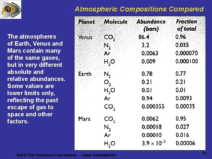
Atmospheric Compositions Compared The atmospheres of Earth, Venus and Mars contain many of the same gases, but in very different absolute and relative abundances. Some values are lower limits only, reflecting the past escape of gas to space and other factors. ASEN 5335 Aerospace Environment -- Upper Atmospheres 52

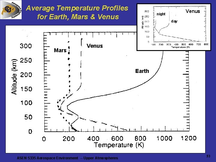
Average Temperature Profiles for Earth, Mars & Venus Mars Venus night day Venus Earth ASEN 5335 Aerospace Environment -- Upper Atmospheres 53

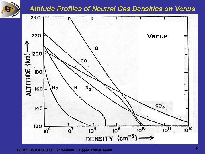
Altitude Profiles of Neutral Gas Densities on Venus ASEN 5335 Aerospace Environment -- Upper Atmospheres 54

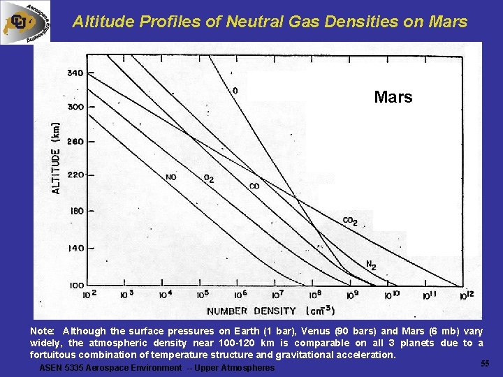
Altitude Profiles of Neutral Gas Densities on Mars Note: Although the surface pressures on Earth (1 bar), Venus (90 bars) and Mars (6 mb) vary widely, the atmospheric density near 100 -120 km is comparable on all 3 planets due to a fortuitous combination of temperature structure and gravitational acceleration. ASEN 5335 Aerospace Environment -- Upper Atmospheres 55

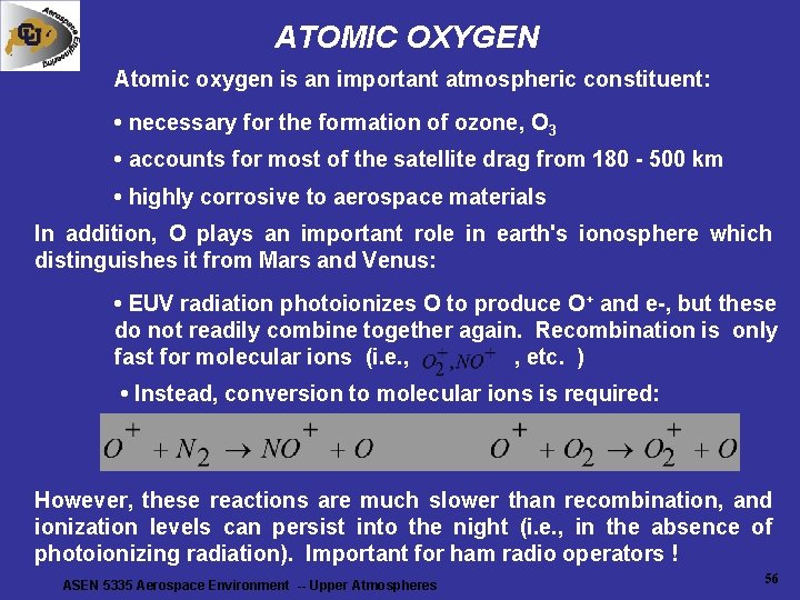
ATOMIC OXYGEN Atomic oxygen is an important atmospheric constituent: • necessary for the formation of ozone, O 3 • accounts for most of the satellite drag from 180 - 500 km • highly corrosive to aerospace materials In addition, O plays an important role in earth's ionosphere which distinguishes it from Mars and Venus: • EUV radiation photoionizes O to produce O+ and e-, but these do not readily combine together again. Recombination is only fast for molecular ions (i. e. , , etc. ) • Instead, conversion to molecular ions is required: However, these reactions are much slower than recombination, and ionization levels can persist into the night (i. e. , in the absence of photoionizing radiation). Important for ham radio operators ! ASEN 5335 Aerospace Environment -- Upper Atmospheres 56

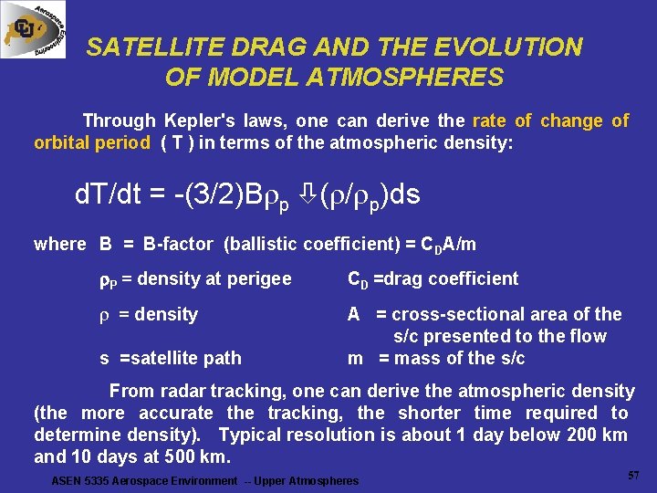
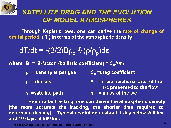
SATELLITE DRAG AND THE EVOLUTION OF MODEL ATMOSPHERES Through Kepler's laws, one can derive the rate of change of orbital period ( T ) in terms of the atmospheric density: d. T/dt = -(3/2)B p ( / p)ds where B = B-factor (ballistic coefficient) = CDA/m r. P = density at perigee CD =drag coefficient = density A = cross-sectional area of the s/c presented to the flow m = mass of the s/c s =satellite path From radar tracking, one can derive the atmospheric density (the more accurate the tracking, the shorter time required to determine density). Typical resolution is about 1 day below 200 km and 10 days at 500 km. ASEN 5335 Aerospace Environment -- Upper Atmospheres 57

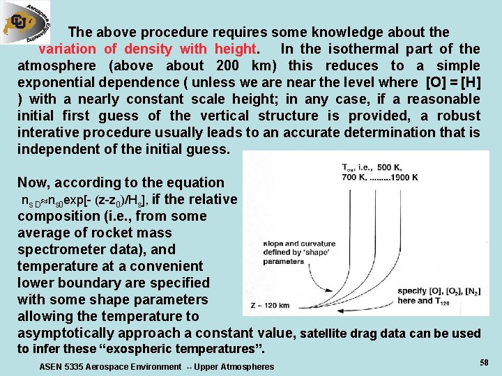
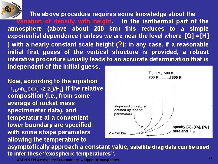
The above procedure requires some knowledge about the variation of density with height. In the isothermal part of the atmosphere (above about 200 km) this reduces to a simple exponential dependence ( unless we are near the level where [O] = [H] ) with a nearly constant scale height; in any case, if a reasonable initial first guess of the vertical structure is provided, a robust interative procedure usually leads to an accurate determination that is independent of the initial guess. Now, according to the equation ns D ns 0 exp[- (z-z 0)/Hs], if the relative composition (i. e. , from some average of rocket mass spectrometer data), and temperature at a convenient lower boundary are specified with some shape parameters allowing the temperature to asymptotically approach a constant value, satellite drag data can be used to infer these “exospheric temperatures”. ASEN 5335 Aerospace Environment -- Upper Atmospheres 58

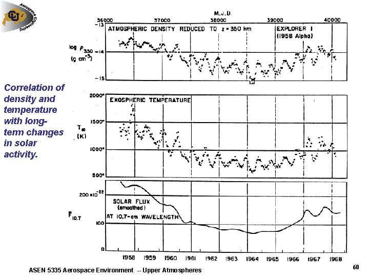
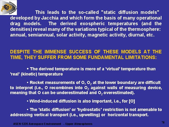
This leads to the so-called "static diffusion models" developed by Jacchia and which form the basis of many operational drag models. The derived exospheric temperatures (and the densities) reveal many of the variations typical of thermosphere: annual, semiannual, solar activity, magnetic activity, diurnal, etc. (see following figures). DESPITE THE IMMENSE SUCCESS OF THESE MODELS AT THE TIME, THEY SUFFER FROM SOME FUNDAMENTAL LIMITATIONS: • The derived temperature is more of a 'virtual' temperature than 'real' (kinetic) temperature • Rocket measurements of O, O 2 at the lower boundary are difficult to interpret (i. e. , O recombines into O 2 against walls of measuring device, meaning that O can be underestimated and O 2 overestimated). • Wind-induced diffusion is also important, i. e. , for [O] • The 'static diffusion' or 'hydrostatic' restriction is not amenable to addressing vertical transport (i. e. , upwelling) or horizontal transport. ASEN 5335 Aerospace Environment -- Upper Atmospheres 59

Correlation of density and temperature with longterm changes in solar activity. ASEN 5335 Aerospace Environment -- Upper Atmospheres 60

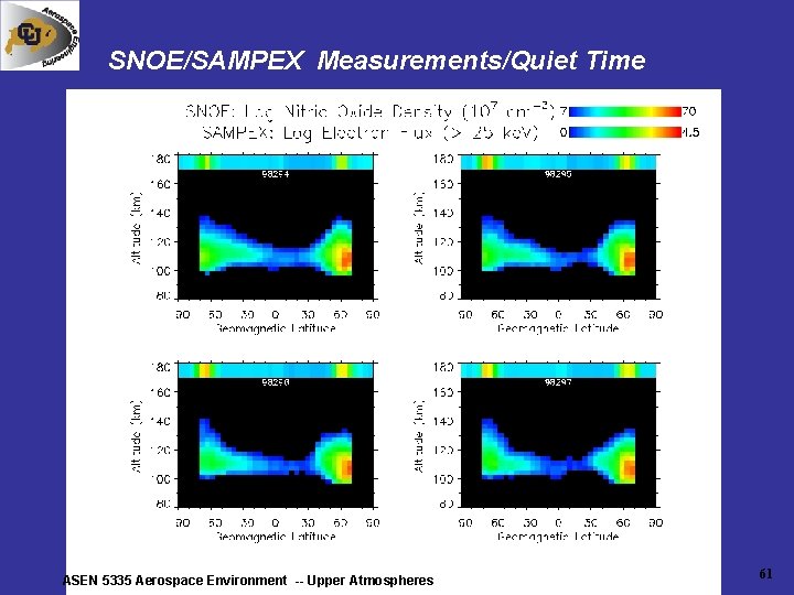
SNOE/SAMPEX Measurements/Quiet Time ASEN 5335 Aerospace Environment -- Upper Atmospheres 61

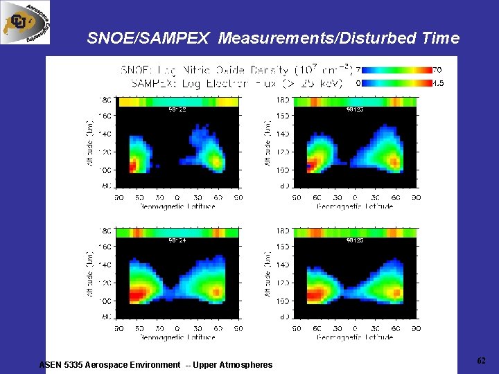
SNOE/SAMPEX Measurements/Disturbed Time ASEN 5335 Aerospace Environment -- Upper Atmospheres 62

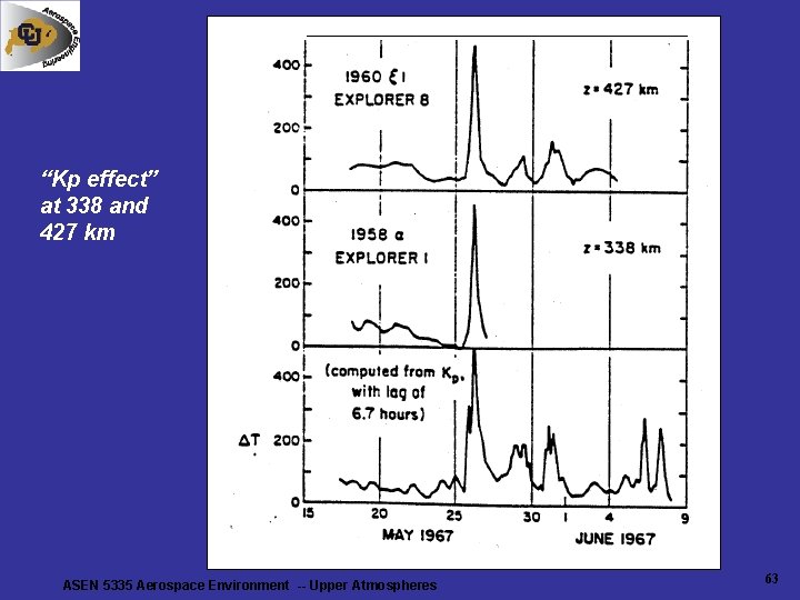
“Kp effect” at 338 and 427 km ASEN 5335 Aerospace Environment -- Upper Atmospheres 63

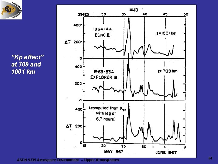
“Kp effect” at 709 and 1001 km ASEN 5335 Aerospace Environment -- Upper Atmospheres 64

Aerospace Environment ASEN-5335 • Instructor: Prof. Xinlin Li (pronounce: Shinlyn Lee) • Contact info: e-mail: lix@lasp. colorado. edu (preferred) phone: 2 -3514, or 5 -0523, fax: 2 -6444, website: http: //lasp. colorado. edu/~lix • Instructor’s office hours: 9 -11 am at ECOT 534 • TA’s office hours: 3: 15 -5: 15 pm Wed at ECAE 166. E-mail: Christopher. Hood@colorado. edu • READ classnotes and Chapter 6 • Quiz-7 on 4/29 • HW 7 due 5/1 ASEN 5335 Aerospace Environment -- Upper Atmospheres 65

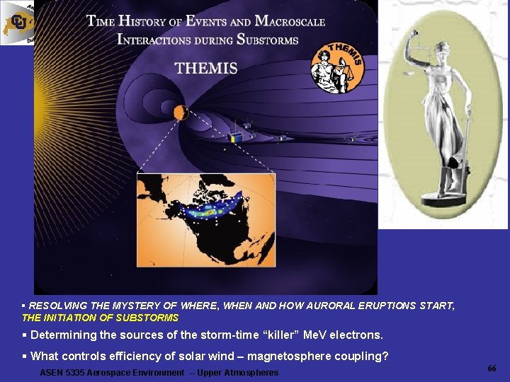
§ RESOLVING THE MYSTERY OF WHERE, WHEN AND HOW AURORAL ERUPTIONS START, THE INITIATION OF SUBSTORMS § Determining the sources of the storm-time “killer” Me. V electrons. § What controls efficiency of solar wind – magnetosphere coupling? ASEN 5335 Aerospace Environment -- Upper Atmospheres 66

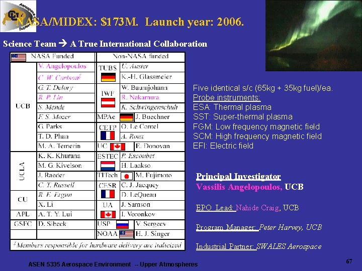
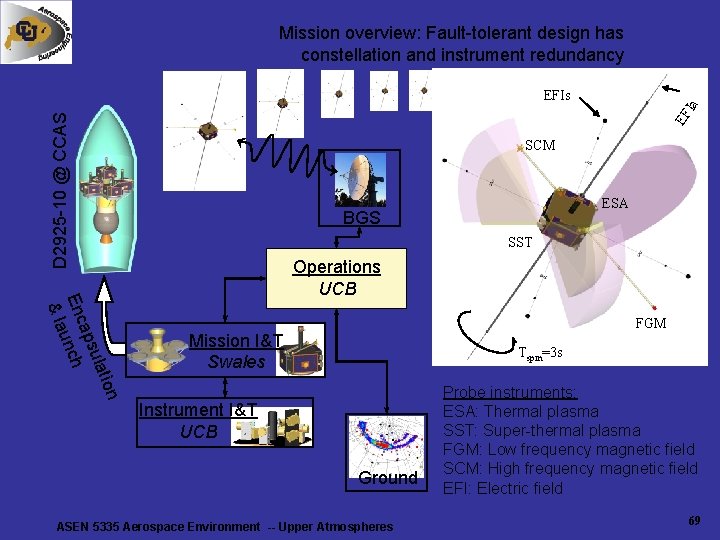
NASA/MIDEX: $173 M. Launch year: 2006. Science Team A True International Collaboration Five identical s/c (65 kg + 35 kg fuel)/ea. Probe instruments: ESA: Thermal plasma SST: Super-thermal plasma FGM: Low frequency magnetic field SCM: High frequency magnetic field EFI: Electric field Principal Investigator Vassilis Angelopoulos, UCB EPO Lead: Nahide Craig, UCB Program Manager: Peter Harvey, UCB Industrial Partner: SWALES Aerospace ASEN 5335 Aerospace Environment -- Upper Atmospheres 67

Events occurring during a substorm Auroral Eruption ASEN 5335 Aerospace Environment -- Upper Atmospheres Current Disruption Reconnection 68

Mission overview: Fault-tolerant design has constellation and instrument redundancy D 2925 -10 @ CCAS EF Ia EFIs SCM ESA BGS SST ion ulat aps Enc unch & la Operations UCB FGM Mission I&T Swales Tspin=3 s Instrument I&T UCB Ground ASEN 5335 Aerospace Environment -- Upper Atmospheres Probe instruments: ESA: Thermal plasma SST: Super-thermal plasma FGM: Low frequency magnetic field SCM: High frequency magnetic field EFI: Electric field 69

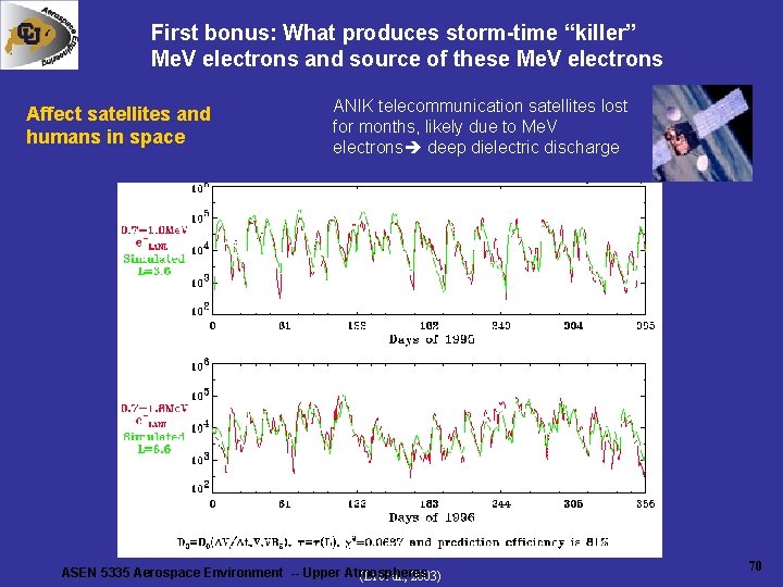
First bonus: What produces storm-time “killer” Me. V electrons and source of these Me. V electrons Affect satellites and humans in space ANIK telecommunication satellites lost for months, likely due to Me. V electrons deep dielectric discharge ASEN 5335 Aerospace Environment -- Upper Atmospheres (Li et al. , 2003) 70

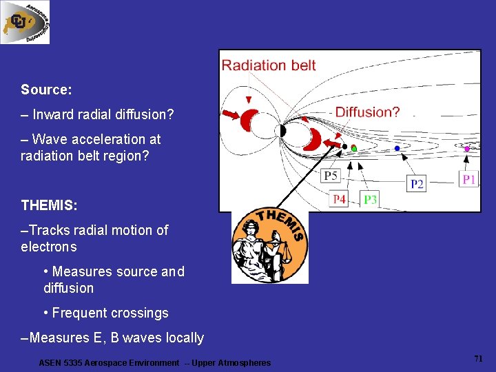
Source: – Inward radial diffusion? – Wave acceleration at radiation belt region? THEMIS: –Tracks radial motion of electrons • Measures source and diffusion • Frequent crossings –Measures E, B waves locally ASEN 5335 Aerospace Environment -- Upper Atmospheres 71

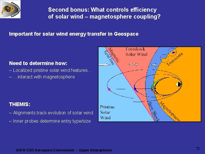
Second bonus: What controls efficiency of solar wind – magnetosphere coupling? Important for solar wind energy transfer in Geospace Need to determine how: – Localized pristine solar wind features… – …interact with magnetosphere THEMIS: – Alignments track evolution of solar wind – Inner probes determine entry type/size ASEN 5335 Aerospace Environment -- Upper Atmospheres 72

Flux Enhance factor Orbit Inclination 25 0. 9 62 1. 09 26 0. 905 88 1. 39 27 0. 91 89 1. 38 28 0. 912 90 1. 37 28. 5 0. 9135 91 1. 38 29 0. 915 92 1. 4 30 0. 92 93 1. 44 31 0. 922 94 1. 5 32 0. 927 95 1. 55 56 1. 06 120 1. 18 57 1. 065 121 1. 165 58 1. 075 122 1. 155 59 1. 08 123 1. 14 60 1. 09 124 1. 125 61 1. 1 ASEN 5335 Aerospace Environment -- Upper Atmospheres 73

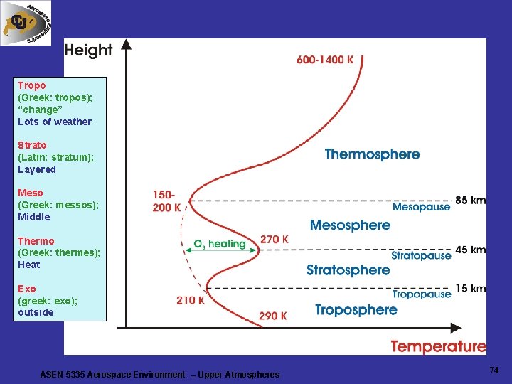
Tropo (Greek: tropos); “change” Lots of weather Strato (Latin: stratum); Layered Meso (Greek: messos); Middle Thermo (Greek: thermes); Heat Exo (greek: exo); outside ASEN 5335 Aerospace Environment -- Upper Atmospheres 74

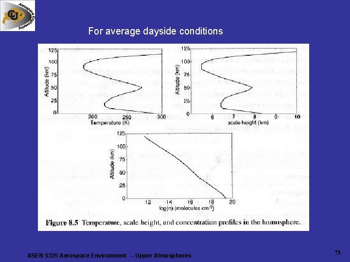
For average dayside conditions ASEN 5335 Aerospace Environment -- Upper Atmospheres 75

SATELLITE DRAG AND THE EVOLUTION OF MODEL ATMOSPHERES Through Kepler's laws, one can derive the rate of change of orbital period ( T ) in terms of the atmospheric density: d. T/dt = -(3/2)B p ( / p)ds where B = B-factor (ballistic coefficient) = CDA/m r. P = density at perigee CD =drag coefficient = density A = cross-sectional area of the s/c presented to the flow m = mass of the s/c s =satellite path From radar tracking, one can derive the atmospheric density (the more accurate the tracking, the shorter time required to determine density). Typical resolution is about 1 day below 200 km and 10 days at 500 km. ASEN 5335 Aerospace Environment -- Upper Atmospheres 76

The above procedure requires some knowledge about the variation of density with height. In the isothermal part of the atmosphere (above about 200 km) this reduces to a simple exponential dependence ( unless we are near the level where [O] = [H] ) with a nearly constant scale height (? ); in any case, if a reasonable initial first guess of the vertical structure is provided, a robust interative procedure usually leads to an accurate determination that is independent of the initial guess. Now, according to the equation ns D ns 0 exp[- (z-z 0)/Hs], if the relative composition (i. e. , from some average of rocket mass spectrometer data), and temperature at a convenient lower boundary are specified with some shape parameters allowing the temperature to asymptotically approach a constant value, satellite drag data can be used to infer these “exospheric temperatures”. ASEN 5335 Aerospace Environment -- Upper Atmospheres 77

This leads to the so-called "static diffusion models" developed by Jacchia and which form the basis of many operational drag models. The derived exospheric temperatures (and the densities) reveal many of the variations typical of thermosphere: annual, semiannual, solar activity, magnetic activity, diurnal, etc. DESPITE THE IMMENSE SUCCESS OF THESE MODELS AT THE TIME, THEY SUFFER FROM SOME FUNDAMENTAL LIMITATIONS: • The derived temperature is more of a 'virtual' temperature than 'real' (kinetic) temperature • Rocket measurements of O, O 2 at the lower boundary are difficult to interpret (i. e. , O recombines into O 2 against walls of measuring device, meaning that O can be underestimated and O 2 overestimated). • Wind-induced diffusion is also important, i. e. , for [O] • The 'static diffusion' or 'hydrostatic' restriction is not amenable to addressing vertical transport (i. e. , upwelling) or horizontal transport. ASEN 5335 Aerospace Environment -- Upper Atmospheres 78

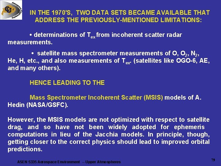
IN THE 1970'S, TWO DATA SETS BECAME AVAILABLE THAT ADDRESS THE PREVIOUSLY-MENTIONED LIMITATIONS: • determinations of Tex from incoherent scatter radar measurements. • satellite mass spectrometer measurements of O, O 2, N 2, He, H, etc. , and also measurements of Tex. (satellites like OGO-6, AE, and many others). HENCE LEADING TO THE Mass Spectrometer Incoherent Scatter (MSIS) models of A. Hedin (NASA/GSFC). However, the MSIS models are not optimized with respect to satellite drag, and so have not been widely adopted for ephemeris computations in lieu of the Jacchia models. In principle, though, getting closer to the correct physics should lead to improved orbital predictions. ASEN 5335 Aerospace Environment -- Upper Atmospheres 79

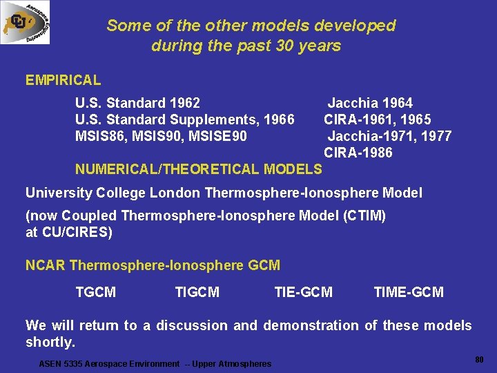
Some of the other models developed during the past 30 years EMPIRICAL U. S. Standard 1962 U. S. Standard Supplements, 1966 MSIS 86, MSIS 90, MSISE 90 Jacchia 1964 CIRA-1961, 1965 Jacchia-1971, 1977 CIRA-1986 NUMERICAL/THEORETICAL MODELS University College London Thermosphere-Ionosphere Model (now Coupled Thermosphere-Ionosphere Model (CTIM) at CU/CIRES) NCAR Thermosphere-Ionosphere GCM TIGCM TIE-GCM TIME-GCM We will return to a discussion and demonstration of these models shortly. ASEN 5335 Aerospace Environment -- Upper Atmospheres 80

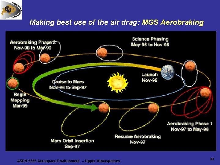
Making best use of the air drag: MGS Aerobraking ASEN 5335 Aerospace Environment -- Upper Atmospheres 81

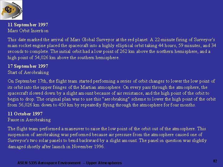
11 September 1997 Mars Orbit Insertion This date marked the arrival of Mars Global Surveyor at the red planet. A 22 -minute firing of Surveyor's main rocket engine placed the spacecraft into a highly elliptical orbit taking 44 hours, 59 minutes, and 34 seconds to complete. The initial orbit had a low point of 262 km above the northern hemisphere, and a high point of 54, 026 km above the southern hemisphere. 17 September 1997 Start of Aerobraking On September 17 th, the flight team started performing a series of orbit changes to lower the low point of its orbit into the upper fringes of the Martian atmosphere. On every pass through the atmosphere, the spacecraft slowed down by a slight amount because of air resistance, and the high point of the orbit to begin to drop. The original plan was to use this "aerobraking" scheme to lower the high point of the orbit from 56, 026 km down to 450 km by repeatedly flying through the atmosphere for four months. 11 October 1997 Pause in Aerobraking The flight team performed a maneuver to raise the low point of the orbit out of the atmosphere. This suspension of aerobraking was performed because air pressure from the atmosphere caused one of Surveyor's two solar panels to bend backward by a slight amount. The panel in question was slightly damaged shortly after launch in November 1996. ASEN 5335 Aerospace Environment -- Upper Atmospheres 82

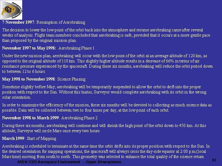
7 November 1997: Resumption of Aerobraking The decision to lower the low point of the orbit back into the atmosphere and resume aerobraking came after several weeks of analysis. Flight team members concluded that aerobraking is safe, provided that it occurs at a more gentle pace than proposed by the original mission plan. November 1997 to May 1998: Aerobraking Phase 1 Under the new mission plan, aerobraking will occur with the low point of the orbit at an average altitude of 120 km, as opposed to the original altitude of 110 km. This slightly higher altitude results in a decrease of 66% in terms of air resistance pressure experienced by the spacecraft. During these six months, aerobraking will reduce the orbit period down to between 12 to 6 hours. May 1998 to November 1998: Science Phasing Sometime slightly before May, aerobraking will be temporarily suspended to allow the orbit to drift into the proper position with respect to the Sun. Without this hiatus, Surveyor would complete aerobraking with its orbit in the wrong solar orientation. In order to maximize the efficiency of the mission, these six months will be devoted to collecting as much science data as possible. Data will be collected between two to four times per day, at the low point of each orbit. November 1998 to March 1999: Aerobraking Phase 2 During these six months, aerobraking will continue and will shrink the high point of the orbit down to 450 km. At this altitude, Surveyor will circle Mars once every two hours. March 1999: Start of Mapping Aerobraking is scheduled to terminate at the same time the orbit drifts into its proper position with respect to the Sun. In the desired orientation for mapping operations, the spacecraft will always cross the day-side equator at 2: 00 p. m. (local Mars time) moving from south to north. This geometry was selected to enhance the total quality of the science return ASEN 5335 Aerospace Environment -- Upper Atmospheres 83

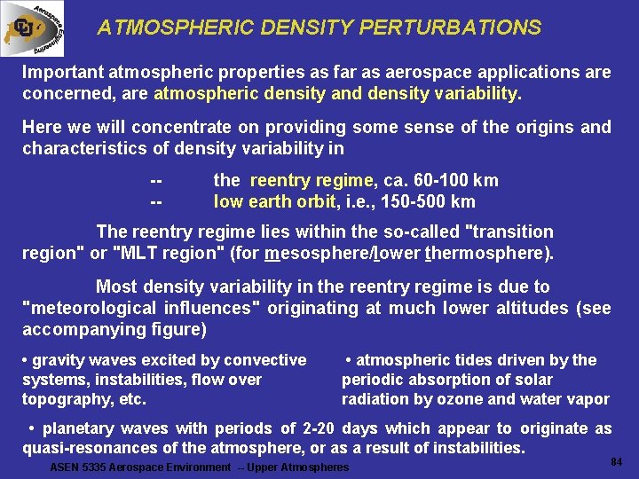
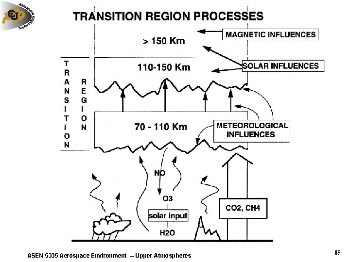
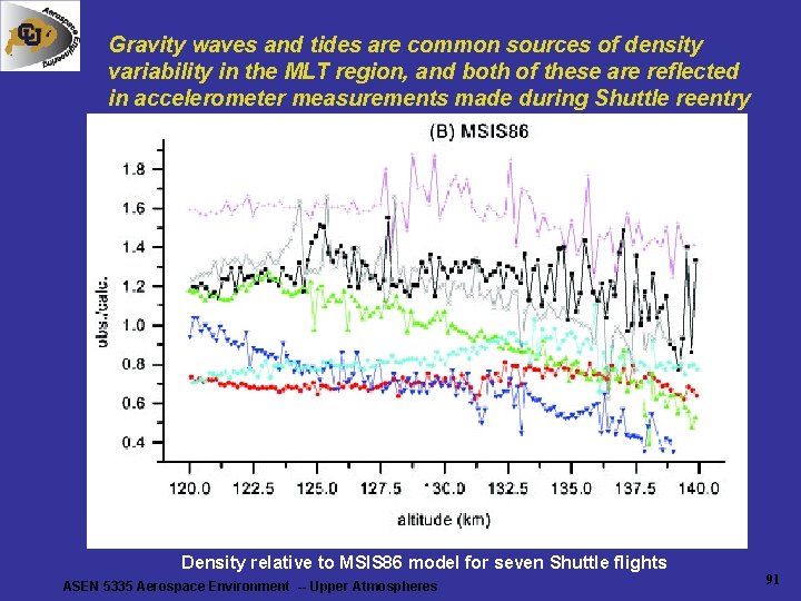
ATMOSPHERIC DENSITY PERTURBATIONS Important atmospheric properties as far as aerospace applications are concerned, are atmospheric density and density variability. Here we will concentrate on providing some sense of the origins and characteristics of density variability in --- the reentry regime, ca. 60 -100 km low earth orbit, i. e. , 150 -500 km The reentry regime lies within the so-called "transition region" or "MLT region" (for mesosphere/lower thermosphere). Most density variability in the reentry regime is due to "meteorological influences" originating at much lower altitudes (see accompanying figure) • gravity waves excited by convective systems, instabilities, flow over topography, etc. • atmospheric tides driven by the periodic absorption of solar radiation by ozone and water vapor • planetary waves with periods of 2 -20 days which appear to originate as quasi-resonances of the atmosphere, or as a result of instabilities. ASEN 5335 Aerospace Environment -- Upper Atmospheres 84

ASEN 5335 Aerospace Environment -- Upper Atmospheres 85

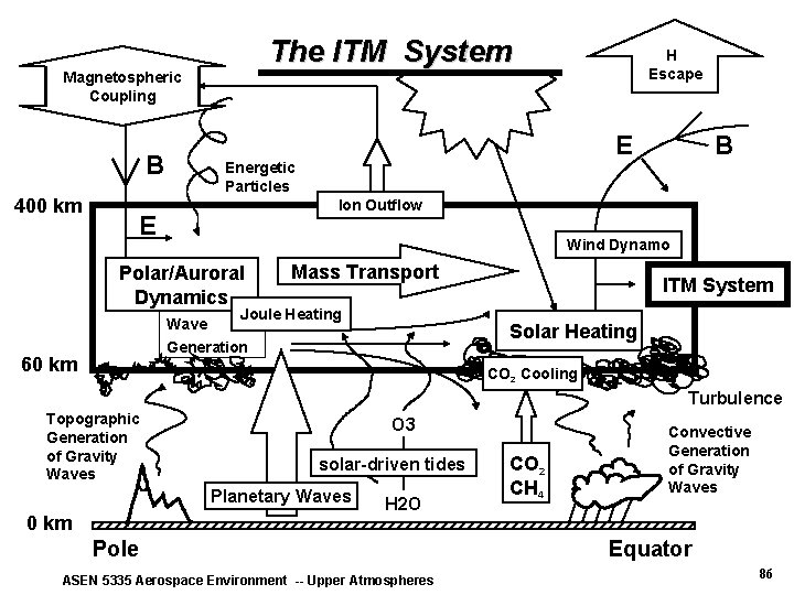
The ITM System Magnetospheric Coupling B 400 km E Energetic Particles B Ion Outflow E Wind Dynamo Polar/Auroral Dynamics Mass Transport Joule Heating Wave Generation 60 km H Escape ITM System Solar Heating CO 2 Cooling Turbulence Topographic Generation of Gravity Waves O 3 solar-driven tides Planetary Waves 0 km H 2 O Pole ASEN 5335 Aerospace Environment -- Upper Atmospheres CO 2 CH 4 Convective Generation of Gravity Waves Equator 86

ASEN 5335 Aerospace Environment -- Upper Atmospheres 87

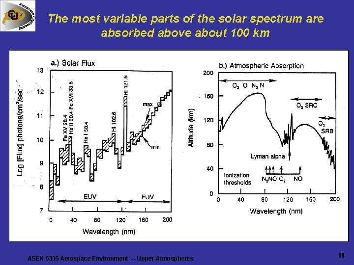
The most variable parts of the solar spectrum are absorbed above about 100 km ASEN 5335 Aerospace Environment -- Upper Atmospheres 88

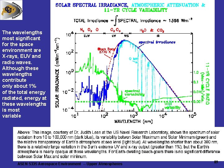
The wavelengths most significant for the space environment are X-rays, EUV and radio waves. Although these wavelengths contribute only about 1% of the total energy radiated, energy at these wavelengths is most variable ASEN 5335 Aerospace Environment -- Upper Atmospheres 89

ASEN 5335 Aerospace Environment -- Upper Atmospheres 90

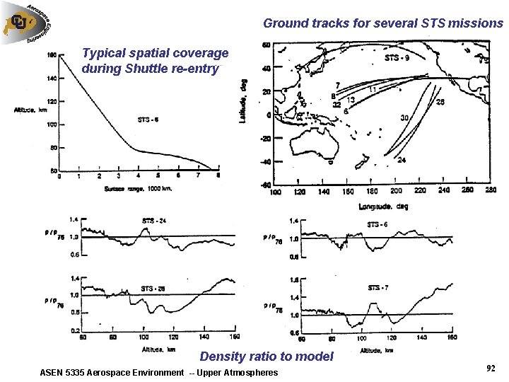
Gravity waves and tides are common sources of density variability in the MLT region, and both of these are reflected in accelerometer measurements made during Shuttle reentry Density relative to MSIS 86 model for seven Shuttle flights ASEN 5335 Aerospace Environment -- Upper Atmospheres 91

Ground tracks for several STS missions Typical spatial coverage during Shuttle re-entry Density ratio to model ASEN 5335 Aerospace Environment -- Upper Atmospheres 92

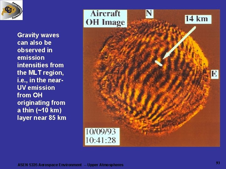
Gravity waves can also be observed in emission intensities from the MLT region, i. e. , in the near. UV emission from OH originating from a thin (~10 km) layer near 85 km ASEN 5335 Aerospace Environment -- Upper Atmospheres 93

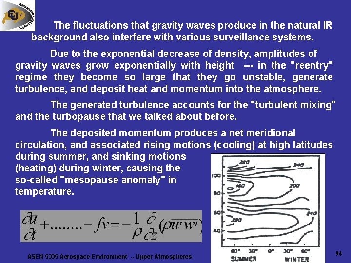
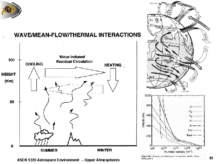
The fluctuations that gravity waves produce in the natural IR background also interfere with various surveillance systems. Due to the exponential decrease of density, amplitudes of gravity waves grow exponentially with height --- in the "reentry" regime they become so large that they go unstable, generate turbulence, and deposit heat and momentum into the atmosphere. The generated turbulence accounts for the "turbulent mixing" and the turbopause that we talked about before. The deposited momentum produces a net meridional circulation, and associated rising motions (cooling) at high latitudes during summer, and sinking motions (heating) during winter, causing the so-called "mesopause anomaly" in temperature. ASEN 5335 Aerospace Environment -- Upper Atmospheres 94

ASEN 5335 Aerospace Environment -- Upper Atmospheres 95

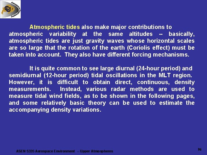
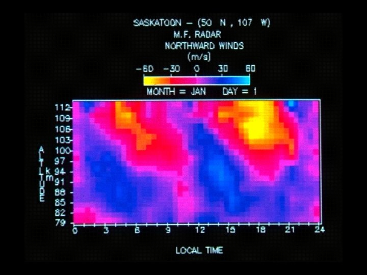
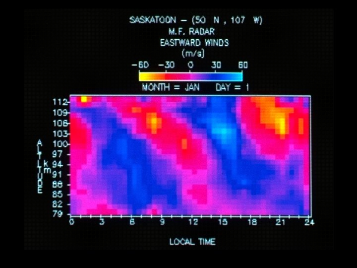
Atmospheric tides also make major contributions to atmospheric variability at the same altitudes -- basically, atmospheric tides are just gravity waves whose horizontal scales are so large that the rotation of the earth (Coriolis effect) must be taken into account. They also have different forcing mechanisms. It is quite common to see large diurnal (24 -hour period) and semidiurnal (12 -hour period) tidal oscillations in the MLT region. However, it is difficult to obtain direct, continuous, density measurements. Instead, various radar methods are used to measure tidal wind fields, as to be shown in the following pages, and some relatively basic theory can be used to estimate the accompanying density variations. ASEN 5335 Aerospace Environment -- Upper Atmospheres 96

ASEN 5335 Aerospace Environment -- Upper Atmospheres 97

ASEN 5335 Aerospace Environment -- Upper Atmospheres 98

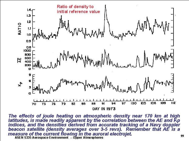
Ratio of density to initial reference value The effects of joule heating on atmospheric density near 170 km at high latitudes, is made readily apparent by the correlation between the AE and Kp indices, and the densities derived from accurate tracking of a Navy doppler beacon satellite (density averages over 3 -5 revs). Remember that AE is a measure of the current flowing in the auroral electrojet. 99 ASEN 5335 Aerospace Environment -- Upper Atmospheres

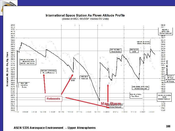
Reboosts Mag Storm ASEN 5335 Aerospace Environment -- Upper Atmospheres 100

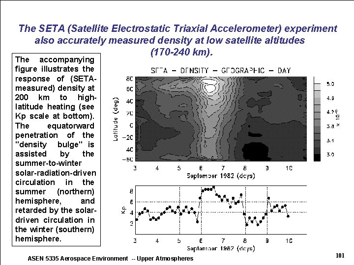
The SETA (Satellite Electrostatic Triaxial Accelerometer) experiment also accurately measured density at low satellite altitudes (170 -240 km). The accompanying figure illustrates the response of (SETAmeasured) density at 200 km to highlatitude heating (see Kp scale at bottom). The equatorward penetration of the "density bulge" is assisted by the summer-to-winter solar-radiation-driven circulation in the summer (northern) hemisphere, and retarded by the solardriven circulation in the winter (southern) hemisphere. ASEN 5335 Aerospace Environment -- Upper Atmospheres 101

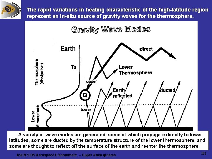
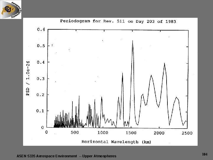
The rapid variations in heating characteristic of the high-latitude region represent an in-situ source of gravity waves for thermosphere. A variety of wave modes are generated, some of which propagate directly to lower latitudes, some are ducted by the temperature structure of the lower thermosphere, and some are thought to reflect off the surface of the earth and reenter thermosphere ASEN 5335 Aerospace Environment -- Upper Atmospheres 102

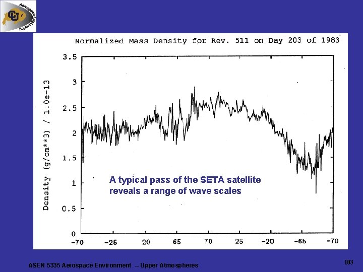
A typical pass of the SETA satellite reveals a range of wave scales ASEN 5335 Aerospace Environment -- Upper Atmospheres 103

ASEN 5335 Aerospace Environment -- Upper Atmospheres 104

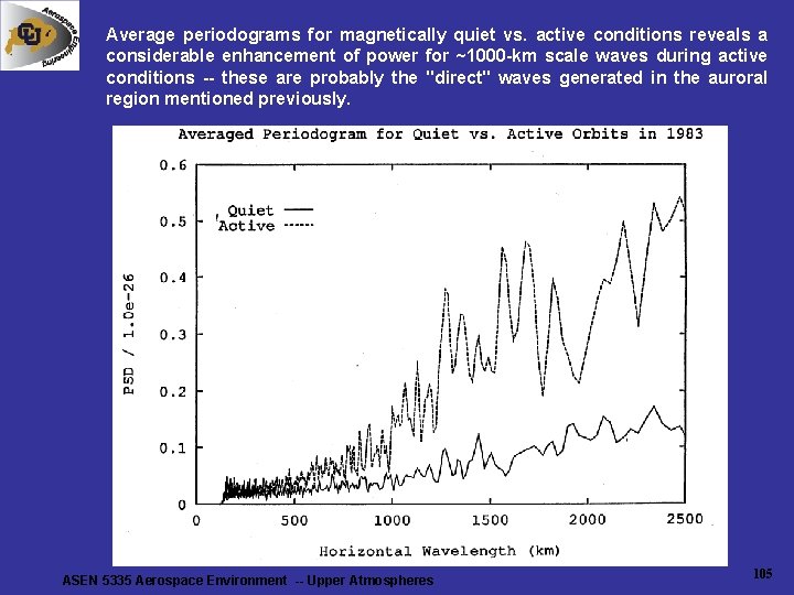
Average periodograms for magnetically quiet vs. active conditions reveals a considerable enhancement of power for ~1000 -km scale waves during active conditions -- these are probably the "direct" waves generated in the auroral region mentioned previously. ASEN 5335 Aerospace Environment -- Upper Atmospheres 105