Magnetic Properties of Complexes Paramagnetism In a paramagnet


 field The energy")


 formula")


- Slides: 26
Magnetic Properties of Complexes
Paramagnetism In a paramagnet, the magnetic moments tend to be randomly orientated due to thermal fluctuations when there is no magnetic field. In an applied magnetic field these moments start to align parallel to the field such that the magnetisation of the material is proportional to the applied field
Magnetic properties Paramagnetism arises from unpaired electrons Each electron has a magnetic moment with one component associated with the spin angular momentum of the electron and (except when the quantum number l = 0) a second component associated with the orbital angular momentum For many complexes of first row d-block metal ions we can ignore the second component and the magnetic moment, , can be regarded as being determined by the number of unpaired electrons, n S
The effective magnetic moment, eff, can be obtained from the experimentally measured molar magnetic susceptibility, m, and is expressed in Bohr magnetons ( B) where 1 B = eh/4 pme = 9. 27 10– 24 JT– 1. The following equations give the relationship between eff and m In SI unit In cgs unit m in cm 3/mol where k = Boltzmann constant L = Avogadro number 0 = vacuum permeability T = temperature in kelvin
By no means do all paramagnetic complexes obey the spin only formula
The states of an ion split in an electric (or ligand) field The energy difference between adjacent states with J values of J’ and (J’ + 1) is given by the expression (J’ + 1) where is called the spin–orbit coupling constant
For the d 2 configuration In a magnetic field, each state with a different J value splits again to give (2 J+1) different levels separated by g. J BB 0 where g. J is a constant called the Lande´ splitting factor and B 0 is the magnetic field
The value of varies from a fraction of a cm– 1 for the very lightest atoms to a few thousand cm– 1 for the heaviest ones The extent to which states of different J values are populated at ambient temperature depends on how large their separation is compared with thermal energy available, k. T; at 300 K, k. T 200 cm– 1 or 2. 6 k. J mol– 1 It can be shown theoretically that if the separation of energy levels is large, the magnetic moment is given by equation
Strictly, this applies only to free-ion energy levels, but it gives values for the magnetic moments of lanthanoid ions (for which is typically 1000 cm– 1) that are in good agreement with observed values
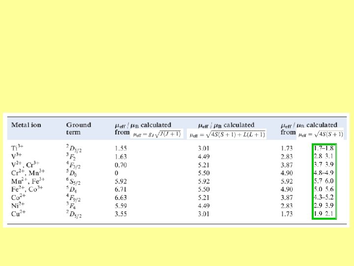
For d-block metal ions, the above equation gives results that correlate poorly with experimental data For many (but not all) first row metal ions, is very small and the spin and orbital angular momenta of the electrons operate independently in the free ion And in a d-block metal complex ion, the crystal field partly or fully quenches the orbital angular momentum For the case where spin and orbital moments do not couple, the van Vleck formula has been derived S+L If there is no contribution from orbital motion, then the Van Vleck equation reduces to the spin-only formula we met earlier
Orbital Contribution In order for an electron to have orbital angular momentum, it must be possible to transform the orbital it occupies into an entirely equivalent and degenerate orbital by rotation The electron is then effectively rotating about the axis used for the rotation of the orbitals
In an octahedral complex, for example, the three t 2 g orbitals can be interconverted by rotations through 900; thus, an electron in a t 2 g orbital has orbital angular momentum The eg orbitals, having different shapes, cannot be interconverted and so electrons in eg orbitals never have angular momentum
There is, however, another factor that needs to be taken into account: if all the t 2 g orbitals are singly occupied, an electron in, say, the dxz orbital cannot be transferred into the dxy or dyz orbital because these already contain an electron having the same spin quantum number as the incoming electron If all the t 2 g orbitals are doubly occupied, electron transfer is also impossible It follows that in high-spin octahedral complexes, orbital contributions to the magnetic moment are important only for the configurations t 2 g 1, t 2 g 2, t 2 g 4 eg 2 and t 2 g 5 eg 2
For tetrahedral complexes, it is similarly shown that the configurations that give rise to an orbital contribution are e 2 t 2 1 , e 2 t 2 2 , e 4 t 2 4 and e 4 t 25
These results lead us to the conclusion that an octahedral high-spin d 7 complex (t 2 g 5 eg 2) should have a magnetic moment greater than the spin-only value of 3. 87 B but a tetrahedral d 7 complex (e 4 t 23) should not However, the observed values of eff for [Co(H 2 O)6]2+ and [Co. Cl 4]2– are 5. 0 and 4. 4 B respectively, i. e. both complexes have magnetic moments greater than (spin-only) The third factor involved is spin–orbit coupling.
Spin-Orbit Coupling Spin–orbit coupling brings us the following equation; this modifies the (spin-only) formula to take into account spin–orbit coupling and, although dependent on Δoct, applies also to tetrahedral complexes where = spin–orbit coupling constant = constant that depends on the ground term: = 4 for an A ground state, and = 2 for an E ground state
Some values of are given below Note that is positive for less than half-filled shells and negative for shells that are more than half-filled. Thus, spin–orbit coupling leads to:
An important point is that spin–orbit coupling is generally large for second and third row d-block metal ions and this leads to large discrepancies between (spin-only) and observed values of eff The following d 1 complexes’ room temperaturte eff illustrate this clearly: Cis-[Nb. Br 4(NCMe)2] 1. 27 Cis-[Ta. Cl 4(NCMe)2] 0. 45 Both have (spin-only) value of 1. 73 B
The effects of temperature on eff If a complex obeys Curie’s law ( = C/T) then its eff is indedpenant of temperature, since, However, the Curie Law is rarely obeyed and so it is essential to state the temperature at which a value of eff has been measured For second and third row d-block metal ions in particular, quoting only a room temperature value of eff is usually meaningless; when spin–orbit coupling is large, eff is highly dependent on T For a given electronic configuration, the influence of temperature on eff can be seen from a Kotani plot of eff against k. T/ where k is the Boltzmann constant, T is the temperature in K, and is the spin–orbit coupling constant Remember that is small for first row metal ions, is large for a second row metal ion, and is even larger for a third row ion.
Kotani plot for a t 2 g 4 configuration Points to note from these data are: Since the points corresponding to eff(298 K) for the first row metal ions lie on the nearhorizontal part of the curve, changing the temperature has little effect on eff; Since the points relating to eff(298 K) for the heavier metal ions lie on parts of the curve with steep gradients, eff is sensitive to changes in temperature; this is especially true for Os(IV).
Ferromagnetism, antiferromagnetism and ferrimagnetism Whenever we have mentioned magnetic properties so far, we have assumed that metal centres have no interaction with each other This is true for substances where the paramagnetic centres are well separated from each other by diamagnetic species; such systems are said to be magnetically dilute When the paramagnetic species are very close together (as in the bulk metal) or are separated by a species that can transmit magnetic interactions (as in many d-block metal oxides, fluorides and chlorides), the metal centres may interact (couple) with one another
The interaction may give rise to ferromagnetism or antiferromagnetism: Ferromagnetism Antiferromagnetism In a ferromagnetic material, large domains of magnetic dipoles are aligned in the same direction; in an antiferromagnetic material, neighbouring magnetic dipoles are aligned in opposite directions
Ferromagnetism leads to greatly enhanced paramagnetism as in iron metal at temperatures of up to 1041 K (the Curie temperature, TC), above which thermal energy is sufficient to overcome the alignment and normal paramagnetic behaviour prevails Antiferromagnetism occurs below the Neel temperature, TN; as the temperature decreases, less thermal energy is available and the paramagnetic susceptibility falls rapidly
Ferrimagnetism If some moments are systematically aligned so as to oppose others, but relative numbers or relative values of the moments are such as to lead to a finite resultant magnetic moment: this is ferrimagnetism and is represented schematically in the following figure
Antiferromagnetic coupling by the Super-Exchange Mechansim When a bridging ligand facilitates the coupling of electron spins on adjacentmetal centres, the mechanismis one of superexchange This is shown schematically in the following diagram, in which the unpaired metal electrons are represented in red