Lecture Slides Elementary Statistics Tenth Edition and the

Lecture Slides Elementary Statistics Tenth Edition and the Triola Statistics Series by Mario F. Triola Copyright © 2007 Pearson Education, Inc Publishing as Pearson Addison-Wesley. Slide 1

Chapter 8 Hypothesis Testing 8 -1 Overview 8 -2 Basics of Hypothesis Testing 8 -3 Testing a Claim about a Proportion 8 -4 Testing a Claim About a Mean: σ Known 8 -5 Testing a Claim About a Mean: σ Not Known 8 -6 Testing a Claim About a Standard Deviation or Variance Slide 2

Section 8 -1 Overview Created by Erin Hodgess, Houston, Texas Revised to accompany 10 th Edition, Tom Wegleitner, Centreville, VA Slide 3

Definitions In statistics, a hypothesis is a claim or statement about a property of a population. A hypothesis test (or test of significance) is a standard procedure for testing a claim about a property of a population. Copyright © 2007 Pearson Education, Inc Publishing as Pearson Addison-Wesley. Slide 4

Rare Event Rule for Inferential Statistics If, under a given assumption, the probability of a particular observed event is exceptionally small, we conclude that the assumption is probably not correct. Copyright © 2007 Pearson Education, Inc Publishing as Pearson Addison-Wesley. Slide 5

Example: Pro. Care Industries, Ltd. , once provided a product called “Gender Choice, ” which, according to advertising claims, allowed couples to “increase your chances of having a boy up to 85%, a girl up to 80%. ” Gender Choice was available in blue packages for couples wanting a baby boy and (you guessed it) pink packages for couples wanting a baby girl. Suppose we conduct an experiment with 100 couples who want to have baby girls, and they all follow the Gender Choice “easy-to-use in-home system” described in the pink package. For the purpose of testing the claim of an increased likelihood for girls, we will assume that Gender Choice has no effect. Using common sense and no formal statistical methods, what should we conclude about the assumption of no effect from Gender Choice if 100 couples using Gender Choice have 100 babies consisting of a) 52 girls? ; b) 97 girls? Slide 6

Example: Pro. Care Industries, Ltd. : Part a) We normally expect around 50 girls in 100 births. The result of 52 girls is close to 50, so we should not conclude that the Gender Choice product is effective. If the 100 couples used no special method of gender selection, the result of 52 girls could easily occur by chance. The assumption of no effect from Gender Choice appears to be correct. There isn’t sufficient evidence to say that Gender Choice is effective. Slide 7

Example: Pro. Care Industries, Ltd. : Part b) The result of 97 girls in 100 births is extremely unlikely to occur by chance. We could explain the occurrence of 97 girls in one of two ways: Either an extremely rare event has occurred by chance, or Gender Choice is effective. The extremely low probability of getting 97 girls is strong evidence against the assumption that Gender Choice has no effect. It does appear to be effective. Slide 8

Section 8 -2 Basics of Hypothesis Testing Created by Erin Hodgess, Houston, Texas Revised to accompany 10 th Edition, Tom Wegleitner, Centreville, VA Slide 9

Key Concept This section presents individual components of a hypothesis test, and the following sections use those components in comprehensive procedures. The role of the following should be understood: v null hypothesis v alternative hypothesis v test statistic v critical region v significance level v critical value v P-value v Type I and II error Copyright © 2007 Pearson Education, Inc Publishing as Pearson Addison-Wesley. Slide 10

Section 8 -2 Objectives v Given a claim, identify the null hypothesis and the alternative hypothesis, and express them both in symbolic form. v Given a claim and sample data, calculate the value of the test statistic. v Given a significance level, identify the critical value(s). v Given a value of the test statistic, identify the P-value. v State the conclusion of a hypothesis test in simple, non-technical terms. Copyright © 2007 Pearson Education, Inc Publishing as Pearson Addison-Wesley. Slide 11

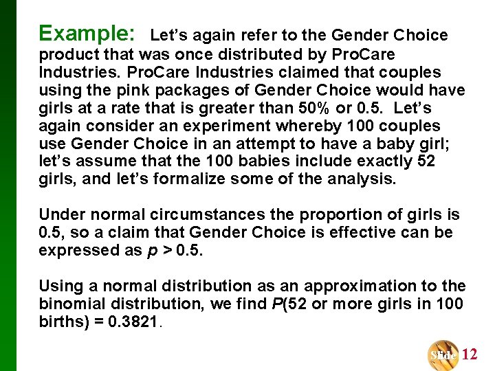
Example: Let’s again refer to the Gender Choice product that was once distributed by Pro. Care Industries claimed that couples using the pink packages of Gender Choice would have girls at a rate that is greater than 50% or 0. 5. Let’s again consider an experiment whereby 100 couples use Gender Choice in an attempt to have a baby girl; let’s assume that the 100 babies include exactly 52 girls, and let’s formalize some of the analysis. Under normal circumstances the proportion of girls is 0. 5, so a claim that Gender Choice is effective can be expressed as p > 0. 5. Using a normal distribution as an approximation to the binomial distribution, we find P(52 or more girls in 100 births) = 0. 3821. Slide 12

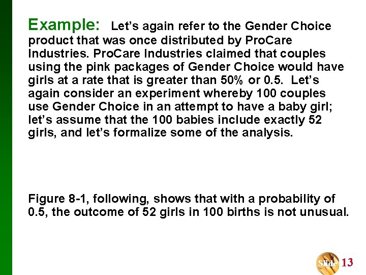
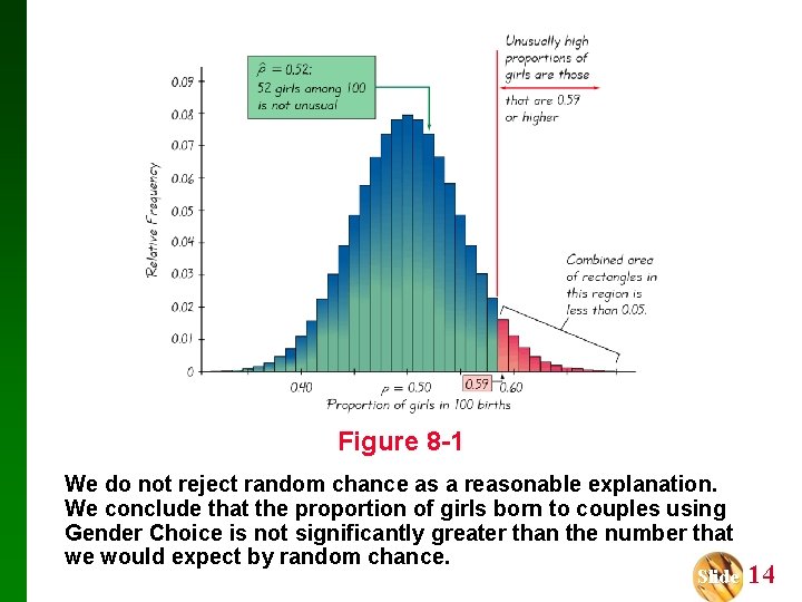
Example: Let’s again refer to the Gender Choice product that was once distributed by Pro. Care Industries claimed that couples using the pink packages of Gender Choice would have girls at a rate that is greater than 50% or 0. 5. Let’s again consider an experiment whereby 100 couples use Gender Choice in an attempt to have a baby girl; let’s assume that the 100 babies include exactly 52 girls, and let’s formalize some of the analysis. Figure 8 -1, following, shows that with a probability of 0. 5, the outcome of 52 girls in 100 births is not unusual. Slide 13

Figure 8 -1 We do not reject random chance as a reasonable explanation. We conclude that the proportion of girls born to couples using Gender Choice is not significantly greater than the number that we would expect by random chance. Slide 14

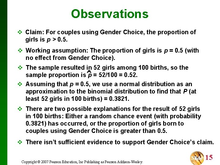
Observations v Claim: For couples using Gender Choice, the proportion of girls is p > 0. 5. v Working assumption: The proportion of girls is p = 0. 5 (with no effect from Gender Choice). v The sample resulted in 52 girls among 100 births, so the sample proportion is p = 52/100 = 0. 52. v Assuming that p = 0. 5, we use a normal distribution as an approximation to the binomial distribution to find that P (at least 52 girls in 100 births) = 0. 3821. ˆ v There are two possible explanations for the result of 52 girls in 100 births: Either a random chance event (with probability 0. 3821) has occurred, or the proportion of girls born to couples using Gender Choice is greater than 0. 5. v There isn’t sufficient evidence to support Gender Choice’s claim. Copyright © 2007 Pearson Education, Inc Publishing as Pearson Addison-Wesley. Slide 15

Components of a Formal Hypothesis Test Copyright © 2007 Pearson Education, Inc Publishing as Pearson Addison-Wesley. Slide 16

Null Hypothesis: H 0 v The null hypothesis (denoted by H 0) is a statement that the value of a population parameter (such as proportion, mean, or standard deviation) is equal to some claimed value. v We test the null hypothesis directly. v Either reject H 0 or fail to reject H 0. Copyright © 2007 Pearson Education, Inc Publishing as Pearson Addison-Wesley. Slide 17

Alternative Hypothesis: H 1 v The alternative hypothesis (denoted by H 1 or Ha or HA) is the statement that the parameter has a value that somehow differs from the null hypothesis. v The symbolic form of the alternative hypothesis must use one of these symbols: , <, >. Copyright © 2007 Pearson Education, Inc Publishing as Pearson Addison-Wesley. Slide 18

Note about Forming Your Own Claims (Hypotheses) If you are conducting a study and want to use a hypothesis test to support your claim, the claim must be worded so that it becomes the alternative hypothesis. Copyright © 2007 Pearson Education, Inc Publishing as Pearson Addison-Wesley. Slide 19

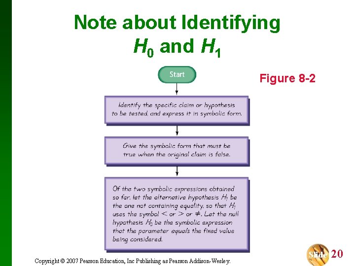
Note about Identifying H 0 and H 1 Figure 8 -2 Copyright © 2007 Pearson Education, Inc Publishing as Pearson Addison-Wesley. Slide 20

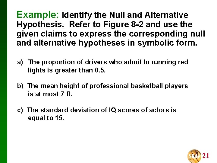
Example: Identify the Null and Alternative Hypothesis. Refer to Figure 8 -2 and use the given claims to express the corresponding null and alternative hypotheses in symbolic form. a) The proportion of drivers who admit to running red lights is greater than 0. 5. b) The mean height of professional basketball players is at most 7 ft. c) The standard deviation of IQ scores of actors is equal to 15. Slide 21

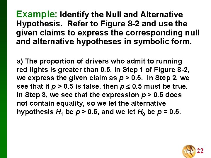
Example: Identify the Null and Alternative Hypothesis. Refer to Figure 8 -2 and use the given claims to express the corresponding null and alternative hypotheses in symbolic form. a) The proportion of drivers who admit to running red lights is greater than 0. 5. In Step 1 of Figure 8 -2, we express the given claim as p > 0. 5. In Step 2, we see that if p > 0. 5 is false, then p 0. 5 must be true. In Step 3, we see that the expression p > 0. 5 does not contain equality, so we let the alternative hypothesis H 1 be p > 0. 5, and we let H 0 be p = 0. 5. Slide 22

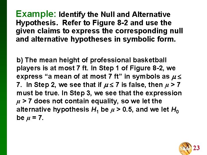
Example: Identify the Null and Alternative Hypothesis. Refer to Figure 8 -2 and use the given claims to express the corresponding null and alternative hypotheses in symbolic form. b) The mean height of professional basketball players is at most 7 ft. In Step 1 of Figure 8 -2, we express “a mean of at most 7 ft” in symbols as 7. In Step 2, we see that if 7 is false, then µ > 7 must be true. In Step 3, we see that the expression µ > 7 does not contain equality, so we let the alternative hypothesis H 1 be µ > 0. 5, and we let H 0 be µ = 7. Slide 23

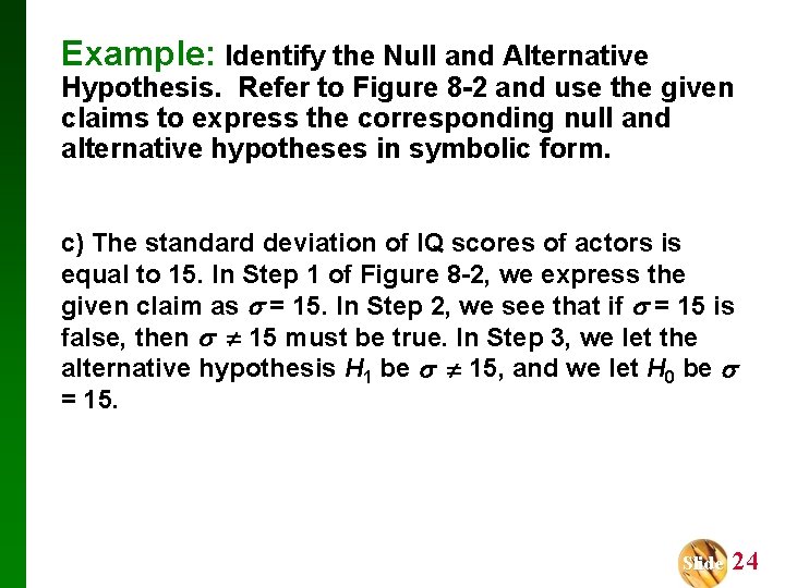
Example: Identify the Null and Alternative Hypothesis. Refer to Figure 8 -2 and use the given claims to express the corresponding null and alternative hypotheses in symbolic form. c) The standard deviation of IQ scores of actors is equal to 15. In Step 1 of Figure 8 -2, we express the given claim as = 15. In Step 2, we see that if = 15 is false, then 15 must be true. In Step 3, we let the alternative hypothesis H 1 be 15, and we let H 0 be = 15. Slide 24

Test Statistic The test statistic is a value used in making a decision about the null hypothesis, and is found by converting the sample statistic to a score with the assumption that the null hypothesis is true. Copyright © 2007 Pearson Education, Inc Publishing as Pearson Addison-Wesley. Slide 25

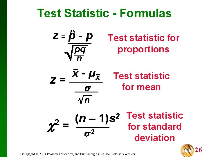
Test Statistic - Formulas z=p-p z = Test statistic for proportions pq n x - µx Test statistic for mean n 2 = (n – 2 1)s 2 Test statistic for standard deviation Copyright © 2007 Pearson Education, Inc Publishing as Pearson Addison-Wesley. Slide 26

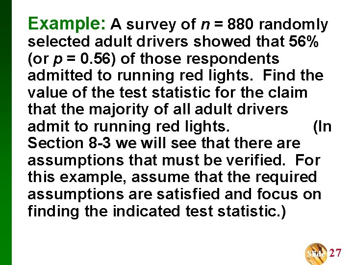
Example: A survey of n = 880 randomly selected adult drivers showed that 56% (or p = 0. 56) of those respondents admitted to running red lights. Find the value of the test statistic for the claim that the majority of all adult drivers admit to running red lights. (In Section 8 -3 we will see that there assumptions that must be verified. For this example, assume that the required assumptions are satisfied and focus on finding the indicated test statistic. ) Slide 27

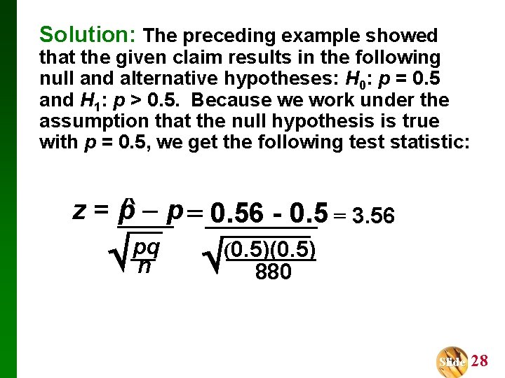
Solution: The preceding example showed that the given claim results in the following null and alternative hypotheses: H 0: p = 0. 5 and H 1: p > 0. 5. Because we work under the assumption that the null hypothesis is true with p = 0. 5, we get the following test statistic: z = p – p = 0. 56 - 0. 5 = 3. 56 pq n (0. 5) 880 Slide 28

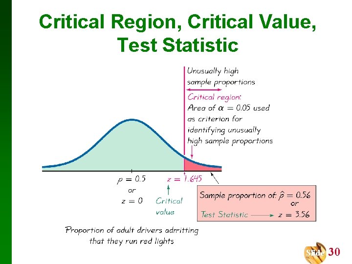
Interpretation: We know from previous chapters that a z score of 3. 56 is exceptionally large. It appears that in addition to being “more than half, ” the sample result of 56% is significantly more than 50%. See figure following. Slide 29

Critical Region, Critical Value, Test Statistic Slide 30

Critical Region The critical region (or rejection region) is the set of all values of the test statistic that cause us to reject the null hypothesis. For example, see the red-shaded region in the previous figure. Copyright © 2007 Pearson Education, Inc Publishing as Pearson Addison-Wesley. Slide 31

Significance Level The significance level (denoted by ) is the probability that the test statistic will fall in the critical region when the null hypothesis is actually true. This is the same introduced in Section 7 -2. Common choices for are 0. 05, 0. 01, and 0. 10. Copyright © 2007 Pearson Education, Inc Publishing as Pearson Addison-Wesley. Slide 32

Critical Value A critical value is any value that separates the critical region (where we reject the null hypothesis) from the values of the test statistic that do not lead to rejection of the null hypothesis. The critical values depend on the nature of the null hypothesis, the sampling distribution that applies, and the significance level . See the previous figure where the critical value of z = 1. 645 corresponds to a significance level of = 0. 05. Copyright © 2007 Pearson Education, Inc Publishing as Pearson Addison-Wesley. Slide 33

Two-tailed, Right-tailed, Left-tailed Tests The tails in a distribution are the extreme regions bounded by critical values. Copyright © 2007 Pearson Education, Inc Publishing as Pearson Addison-Wesley. Slide 34

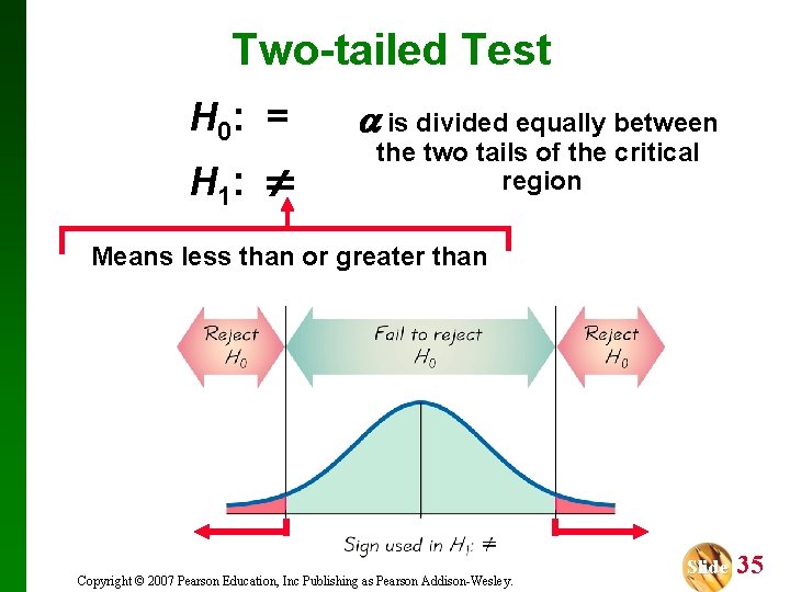
Two-tailed Test H 0: = H 1: is divided equally between the two tails of the critical region Means less than or greater than Copyright © 2007 Pearson Education, Inc Publishing as Pearson Addison-Wesley. Slide 35

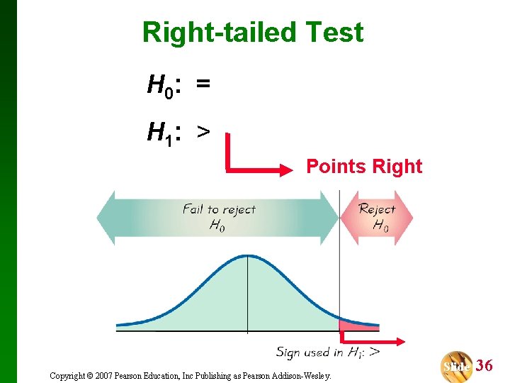
Right-tailed Test H 0: = H 1: > Points Right Copyright © 2007 Pearson Education, Inc Publishing as Pearson Addison-Wesley. Slide 36

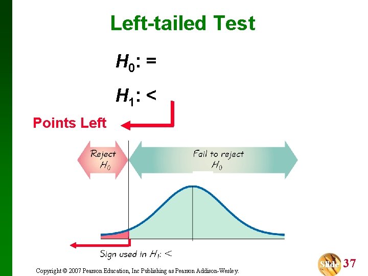
Left-tailed Test H 0: = H 1: < Points Left Copyright © 2007 Pearson Education, Inc Publishing as Pearson Addison-Wesley. Slide 37

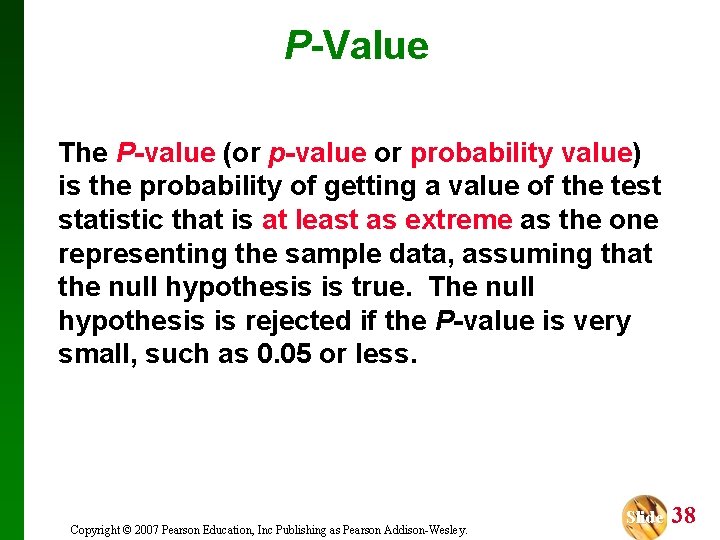
P-Value The P-value (or p-value or probability value) is the probability of getting a value of the test statistic that is at least as extreme as the one representing the sample data, assuming that the null hypothesis is true. The null hypothesis is rejected if the P-value is very small, such as 0. 05 or less. Copyright © 2007 Pearson Education, Inc Publishing as Pearson Addison-Wesley. Slide 38

Conclusions in Hypothesis Testing We always test the null hypothesis. The initial conclusion will always be one of the following: 1. Reject the null hypothesis. 2. Fail to reject the null hypothesis. Copyright © 2007 Pearson Education, Inc Publishing as Pearson Addison-Wesley. Slide 39

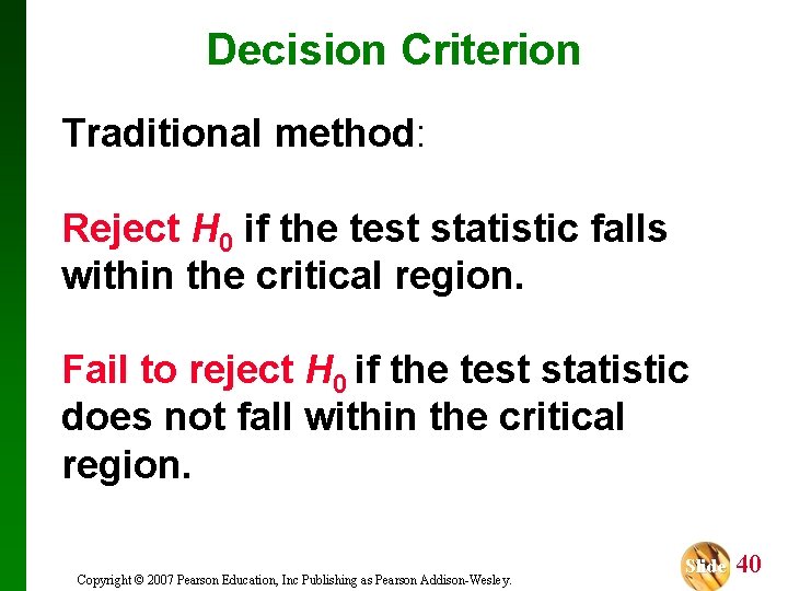
Decision Criterion Traditional method: Reject H 0 if the test statistic falls within the critical region. Fail to reject H 0 if the test statistic does not fall within the critical region. Copyright © 2007 Pearson Education, Inc Publishing as Pearson Addison-Wesley. Slide 40

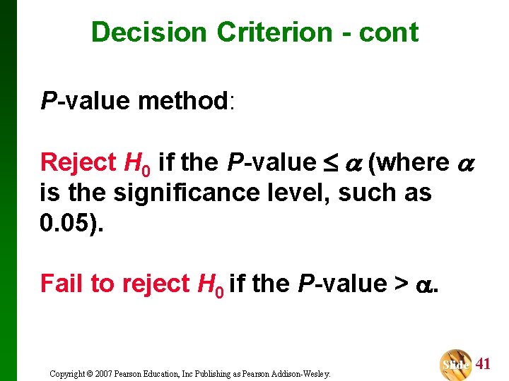
Decision Criterion - cont P-value method: Reject H 0 if the P-value (where is the significance level, such as 0. 05). Fail to reject H 0 if the P-value > . Copyright © 2007 Pearson Education, Inc Publishing as Pearson Addison-Wesley. Slide 41

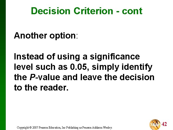
Decision Criterion - cont Another option: Instead of using a significance level such as 0. 05, simply identify the P-value and leave the decision to the reader. Copyright © 2007 Pearson Education, Inc Publishing as Pearson Addison-Wesley. Slide 42

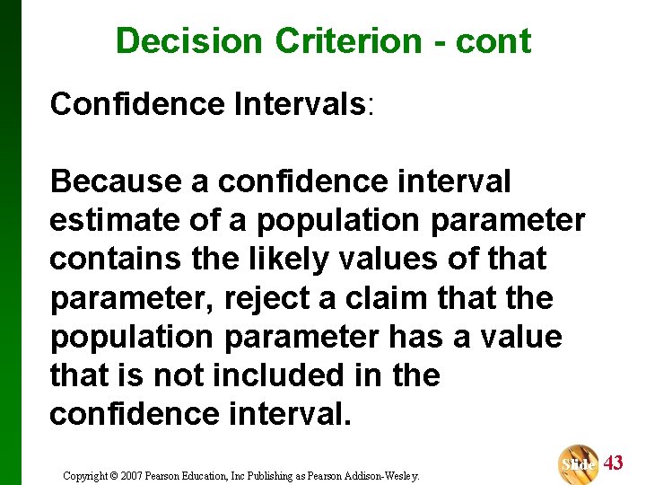
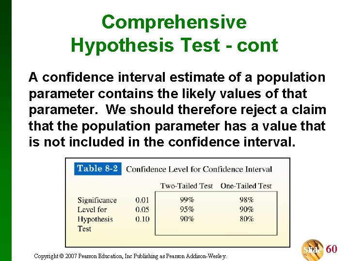
Decision Criterion - cont Confidence Intervals: Because a confidence interval estimate of a population parameter contains the likely values of that parameter, reject a claim that the population parameter has a value that is not included in the confidence interval. Copyright © 2007 Pearson Education, Inc Publishing as Pearson Addison-Wesley. Slide 43

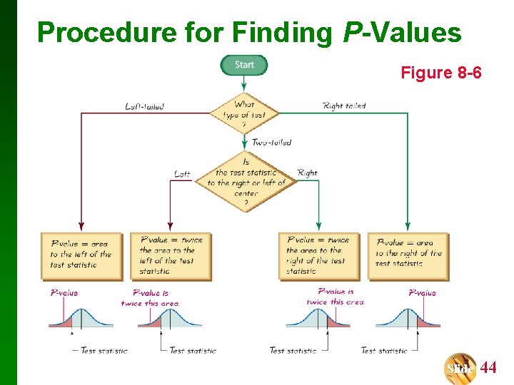
Procedure for Finding P-Values Figure 8 -6 Slide 44

Example: Finding P-values. First determine whether the given conditions result in a righttailed test, a left-tailed test, or a two-tailed test, then find the P-values and state a conclusion about the null hypothesis. a) A significance level of = 0. 05 is used in testing the claim that p > 0. 25, and the sample data result in a test statistic of z = 1. 18. b) A significance level of = 0. 05 is used in testing the claim that p 0. 25, and the sample data result in a test statistic of z = 2. 34. Slide 45

Example: Finding P-values. First determine whether the given conditions result in a righttailed test, a left-tailed test, or a two-tailed test, then find the P-values and state a conclusion about the null hypothesis. a) With a claim of p > 0. 25, the test is right-tailed. Because the test is right-tailed, Figure 8 -6 shows that the P-value is the area to the right of the test statistic z = 1. 18. We refer to Table A-2 and find that the area to the right of z = 1. 18 is 0. 1190. The P-value of 0. 1190 is greater than the significance level = 0. 05, so we fail to reject the null hypothesis. The P-value of 0. 1190 is relatively large, indicating that the sample results could easily occur by chance. Slide 46

Example: Finding P-values. First determine whether the given conditions result in a righttailed test, a left-tailed test, or a two-tailed test, then find the P-values and state a conclusion about the null hypothesis. b) With a claim of p 0. 25, the test is two-tailed. Because the test is two-tailed, and because the test statistic of z = 2. 34 is to the right of the center, Figure 8 -6 shows that the P-value is twice the area to the right of z = 2. 34. We refer to Table A-2 and find that the area to the right of z = 2. 34 is 0. 0096, so P-value = 2 x 0. 0096 = 0. 0192. The P-value of 0. 0192 is less than or equal to the significance level, so we reject the null hypothesis. The small P-value o 0. 0192 shows that the sample results are not likely to occur by chance. Slide 47

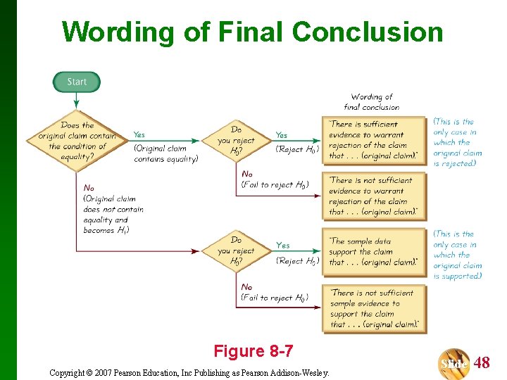
Wording of Final Conclusion Figure 8 -7 Copyright © 2007 Pearson Education, Inc Publishing as Pearson Addison-Wesley. Slide 48

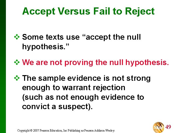
Accept Versus Fail to Reject v Some texts use “accept the null hypothesis. ” v We are not proving the null hypothesis. v The sample evidence is not strong enough to warrant rejection (such as not enough evidence to convict a suspect). Copyright © 2007 Pearson Education, Inc Publishing as Pearson Addison-Wesley. Slide 49

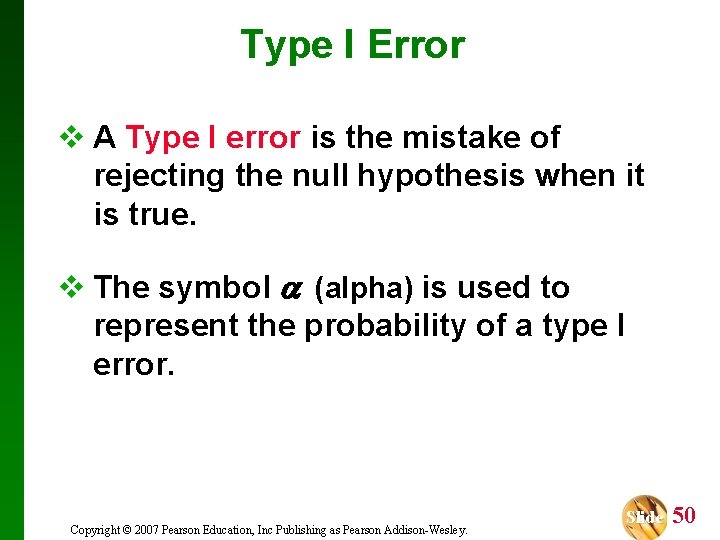
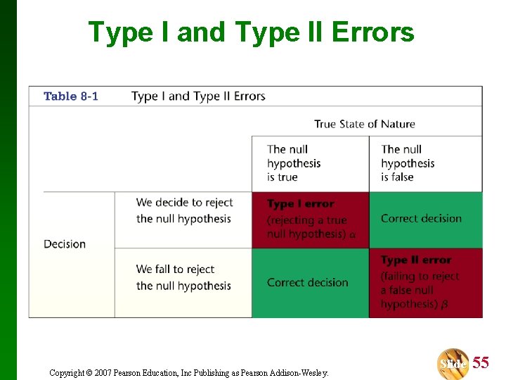
Type I Error v A Type I error is the mistake of rejecting the null hypothesis when it is true. v The symbol (alpha) is used to represent the probability of a type I error. Copyright © 2007 Pearson Education, Inc Publishing as Pearson Addison-Wesley. Slide 50

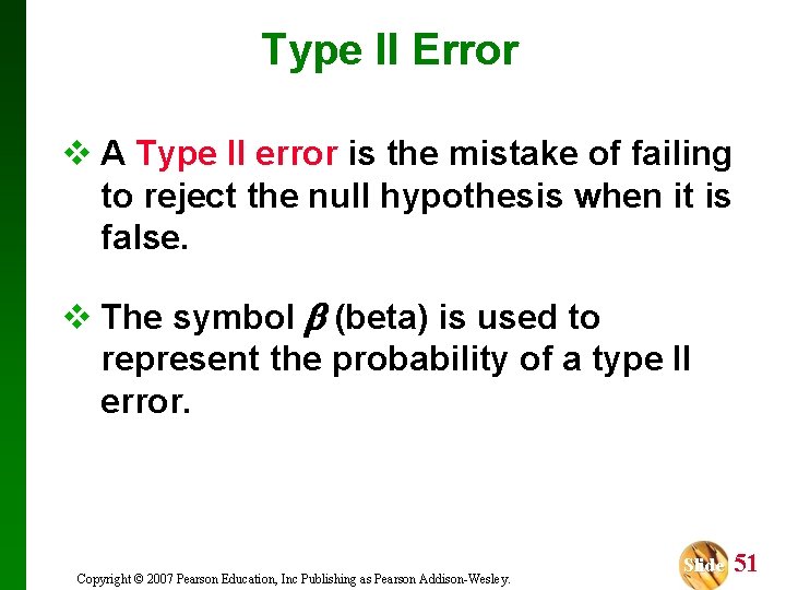
Type II Error v A Type II error is the mistake of failing to reject the null hypothesis when it is false. v The symbol (beta) is used to represent the probability of a type II error. Copyright © 2007 Pearson Education, Inc Publishing as Pearson Addison-Wesley. Slide 51

Example: Assume that we a conducting a hypothesis test of the claim p > 0. 5. Here are the null and alternative hypotheses: H 0: p = 0. 5, and H 1: p > 0. 5. a) Identify a type I error. b) Identify a type II error. Slide 52

Example: Assume that we a conducting a hypothesis test of the claim p > 0. 5. Here are the null and alternative hypotheses: H 0: p = 0. 5, and H 1: p > 0. 5. a) A type I error is the mistake of rejecting a true null hypothesis, so this is a type I error: Conclude that there is sufficient evidence to support p > 0. 5, when in reality p = 0. 5. Slide 53

Example: Assume that we a conducting a hypothesis test of the claim p > 0. 5. Here are the null and alternative hypotheses: H 0: p = 0. 5, and H 1: p > 0. 5. b) A type II error is the mistake of failing to reject the null hypothesis when it is false, so this is a type II error: Fail to reject p = 0. 5 (and therefore fail to support p > 0. 5) when in reality p > 0. 5. Slide 54

Type I and Type II Errors Copyright © 2007 Pearson Education, Inc Publishing as Pearson Addison-Wesley. Slide 55

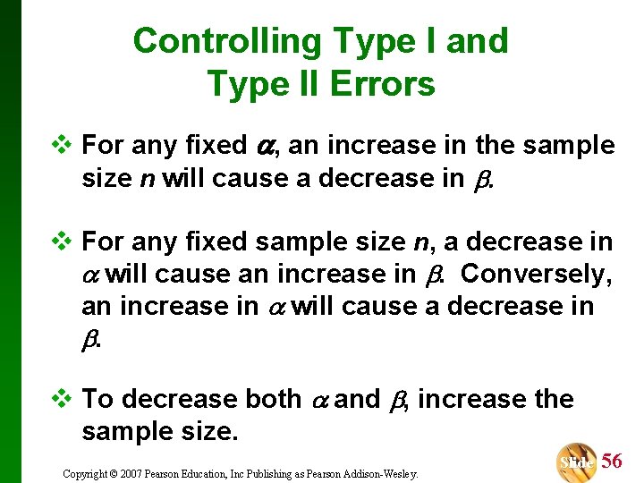
Controlling Type I and Type II Errors v For any fixed , an increase in the sample size n will cause a decrease in v For any fixed sample size n, a decrease in will cause an increase in . Conversely, an increase in will cause a decrease in . v To decrease both and , increase the sample size. Copyright © 2007 Pearson Education, Inc Publishing as Pearson Addison-Wesley. Slide 56

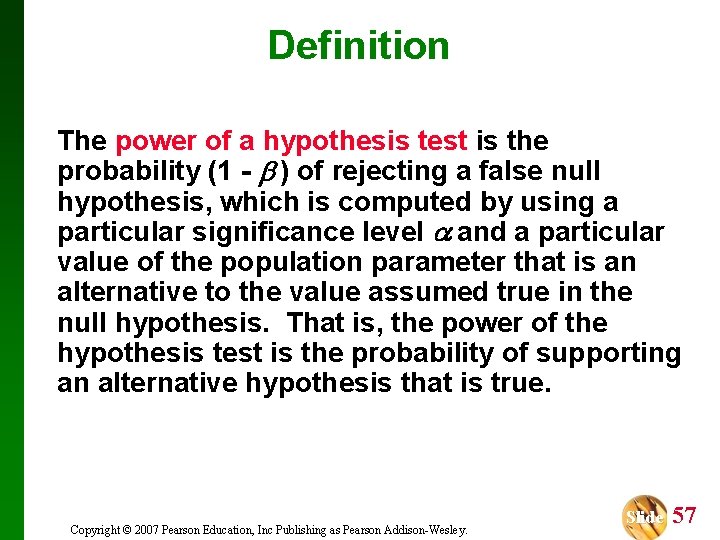
Definition The power of a hypothesis test is the probability (1 - ) of rejecting a false null hypothesis, which is computed by using a particular significance level and a particular value of the population parameter that is an alternative to the value assumed true in the null hypothesis. That is, the power of the hypothesis test is the probability of supporting an alternative hypothesis that is true. Copyright © 2007 Pearson Education, Inc Publishing as Pearson Addison-Wesley. Slide 57

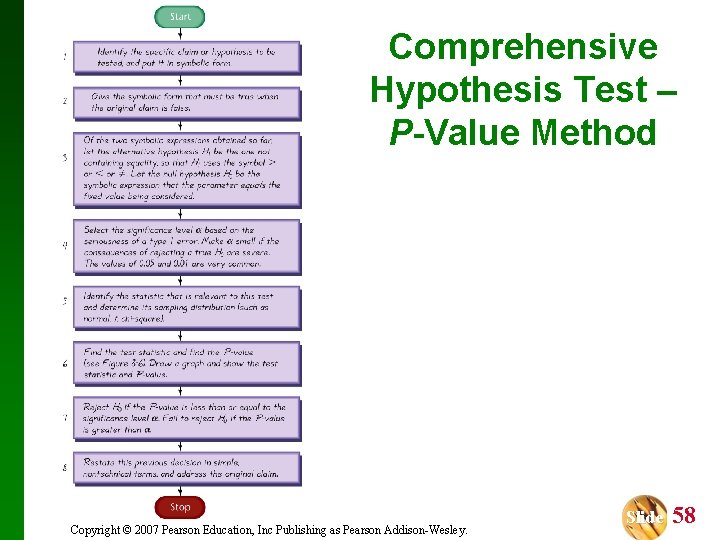
Comprehensive Hypothesis Test – P-Value Method Copyright © 2007 Pearson Education, Inc Publishing as Pearson Addison-Wesley. Slide 58

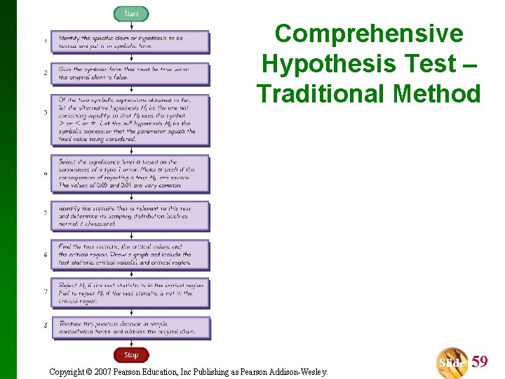
Comprehensive Hypothesis Test – Traditional Method Copyright © 2007 Pearson Education, Inc Publishing as Pearson Addison-Wesley. Slide 59

Comprehensive Hypothesis Test - cont A confidence interval estimate of a population parameter contains the likely values of that parameter. We should therefore reject a claim that the population parameter has a value that is not included in the confidence interval. Copyright © 2007 Pearson Education, Inc Publishing as Pearson Addison-Wesley. Slide 60

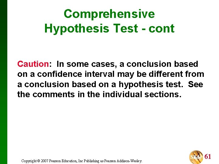
Comprehensive Hypothesis Test - cont Caution: In some cases, a conclusion based on a confidence interval may be different from a conclusion based on a hypothesis test. See the comments in the individual sections. Copyright © 2007 Pearson Education, Inc Publishing as Pearson Addison-Wesley. Slide 61

Recap In this section we have discussed: v Null and alternative hypotheses. v Test statistics. v Significance levels. v P-values. v Decision criteria. v Type I and II errors. v Power of a hypothesis test. Copyright © 2007 Pearson Education, Inc Publishing as Pearson Addison-Wesley. Slide 62

Section 8 -3 Testing a Claim About a Proportion Created by Erin Hodgess, Houston, Texas Revised to accompany 10 th Edition, Tom Wegleitner, Centreville, VA Slide 63

Key Concept This section presents complete procedures for testing a hypothesis (or claim) made about a population proportion. This section uses the components introduced in the previous section for the P-value method, the traditional method or the use of confidence intervals. Copyright © 2007 Pearson Education, Inc Publishing as Pearson Addison-Wesley. Slide 64

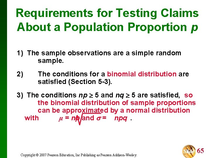
Requirements for Testing Claims About a Population Proportion p 1) The sample observations are a simple random sample. 2) The conditions for a binomial distribution are satisfied (Section 5 -3). 3) The conditions np 5 and nq 5 are satisfied, so the binomial distribution of sample proportions can be approximated by a normal distribution with µ = np and = npq. Copyright © 2007 Pearson Education, Inc Publishing as Pearson Addison-Wesley. Slide 65

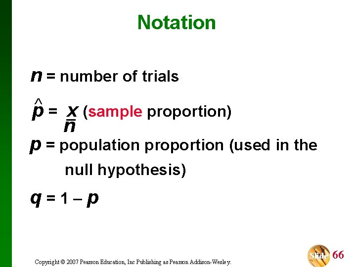
Notation n = number of trials p = x (sample proportion) n p = population proportion (used in the null hypothesis) q = 1 – p Copyright © 2007 Pearson Education, Inc Publishing as Pearson Addison-Wesley. Slide 66

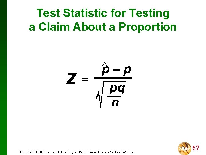
Test Statistic for Testing a Claim About a Proportion z= p–p pq n Copyright © 2007 Pearson Education, Inc Publishing as Pearson Addison-Wesley. Slide 67

P-Value Method Use the same method as described in Section 8 -2 and in Figure 8 -8. Use the standard normal distribution (Table A-2). Copyright © 2007 Pearson Education, Inc Publishing as Pearson Addison-Wesley. Slide 68

Traditional Method Use the same method as described in Section 8 -2 and in Figure 8 -9. Copyright © 2007 Pearson Education, Inc Publishing as Pearson Addison-Wesley. Slide 69

Confidence Interval Method Use the same method as described in Section 8 -2 and in Table 8 -2. Copyright © 2007 Pearson Education, Inc Publishing as Pearson Addison-Wesley. Slide 70

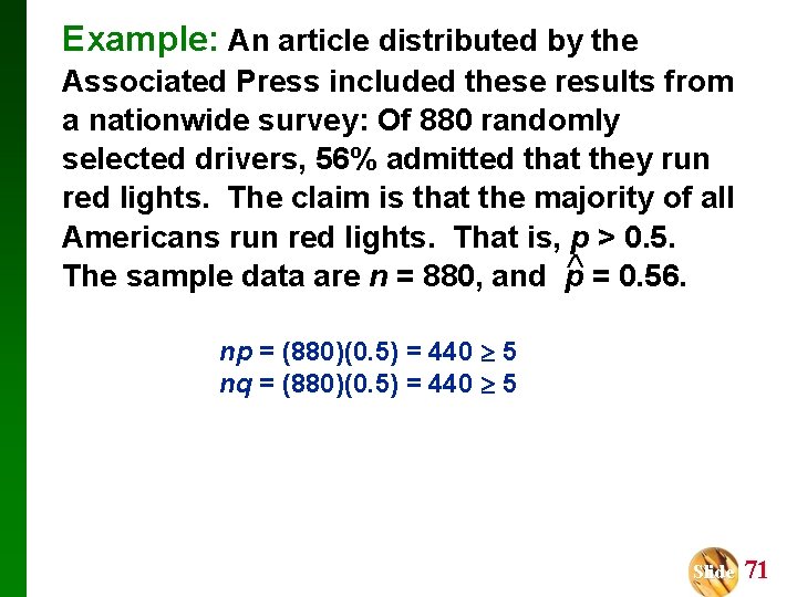
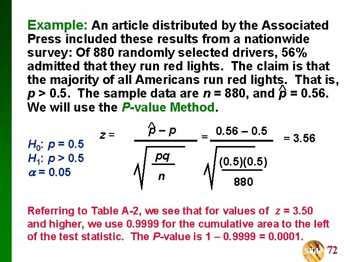
Example: An article distributed by the Associated Press included these results from a nationwide survey: Of 880 randomly selected drivers, 56% admitted that they run red lights. The claim is that the majority of all Americans run red lights. That is, p > 0. 5. The sample data are n = 880, and p = 0. 56. np = (880)(0. 5) = 440 5 nq = (880)(0. 5) = 440 5 Slide 71

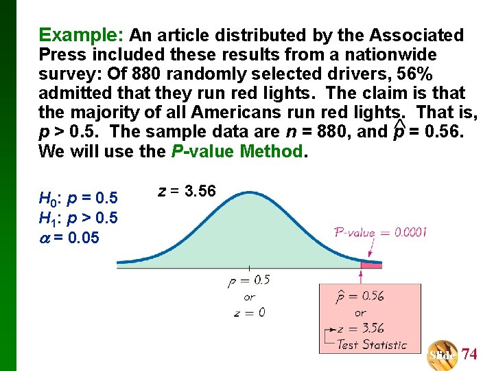
Example: An article distributed by the Associated Press included these results from a nationwide survey: Of 880 randomly selected drivers, 56% admitted that they run red lights. The claim is that the majority of all Americans run red lights. That is, p > 0. 5. The sample data are n = 880, and p = 0. 56. We will use the P-value Method. H 0: p = 0. 5 H 1: p > 0. 5 = 0. 05 z= p–p pq n = 0. 56 – 0. 5 = 3. 56 (0. 5) 880 Referring to Table A-2, we see that for values of z = 3. 50 and higher, we use 0. 9999 for the cumulative area to the left of the test statistic. The P-value is 1 – 0. 9999 = 0. 0001. Slide 72

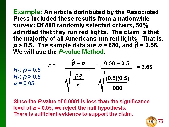
Example: An article distributed by the Associated Press included these results from a nationwide survey: Of 880 randomly selected drivers, 56% admitted that they run red lights. The claim is that the majority of all Americans run red lights. That is, p > 0. 5. The sample data are n = 880, and p = 0. 56. We will use the P-value Method. H 0: p = 0. 5 H 1: p > 0. 5 = 0. 05 z= p–p pq n = 0. 56 – 0. 5 = 3. 56 (0. 5) 880 Since the P-value of 0. 0001 is less than the significance level of = 0. 05, we reject the null hypothesis. There is sufficient evidence to support the claim. Slide 73

Example: An article distributed by the Associated Press included these results from a nationwide survey: Of 880 randomly selected drivers, 56% admitted that they run red lights. The claim is that the majority of all Americans run red lights. That is, p > 0. 5. The sample data are n = 880, and p = 0. 56. We will use the P-value Method. H 0: p = 0. 5 H 1: p > 0. 5 = 0. 05 z = 3. 56 Slide 74

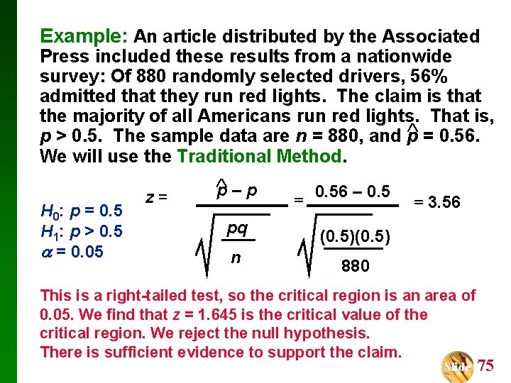
Example: An article distributed by the Associated Press included these results from a nationwide survey: Of 880 randomly selected drivers, 56% admitted that they run red lights. The claim is that the majority of all Americans run red lights. That is, p > 0. 5. The sample data are n = 880, and p = 0. 56. We will use the Traditional Method. H 0: p = 0. 5 H 1: p > 0. 5 = 0. 05 z= p–p pq n = 0. 56 – 0. 5 = 3. 56 (0. 5) 880 This is a right-tailed test, so the critical region is an area of 0. 05. We find that z = 1. 645 is the critical value of the critical region. We reject the null hypothesis. There is sufficient evidence to support the claim. Slide 75

Example: An article distributed by the Associated Press included these results from a nationwide survey: Of 880 randomly selected drivers, 56% admitted that they run red lights. The claim is that the majority of all Americans run red lights. That is, p > 0. 5. The sample data are n = 880, and p = 0. 56. We will use the confidence interval method. For a one-tailed hypothesis test with significance level , we will construct a confidence interval with a confidence level of 1 – 2. We construct a 90% confidence interval. We obtain 0. 533 < p < 0. 588. We are 90% confident that the true value of p is contained within the limits of 0. 533 and 0. 588. Thus we support the claim that p > 0. 5. Slide 76

CAUTION When testing claims about a population proportion, the traditional method and the P-value method are equivalent and will yield the same result since they use the same standard deviation based on the claimed proportion p. However, the confidence interval uses an estimated standard deviation based upon the sample proportion p. Consequently, it is possible that the traditional and P-value methods may yield a different conclusion than the confidence interval method. A good strategy is to use a confidence interval to estimate a population proportion, but use the P-value or traditional method for testing a hypothesis. Copyright © 2007 Pearson Education, Inc Publishing as Pearson Addison-Wesley. Slide 77

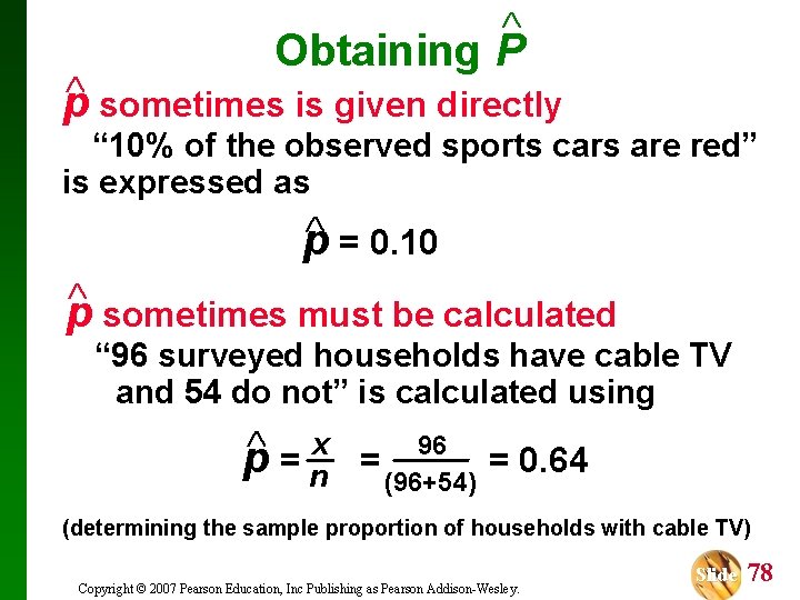
Obtaining P p sometimes is given directly “ 10% of the observed sports cars are red” is expressed as p = 0. 10 p sometimes must be calculated “ 96 surveyed households have cable TV and 54 do not” is calculated using p 96 x = = = 0. 64 n (96+54) (determining the sample proportion of households with cable TV) Copyright © 2007 Pearson Education, Inc Publishing as Pearson Addison-Wesley. Slide 78

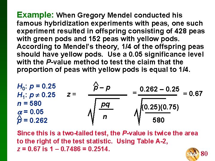
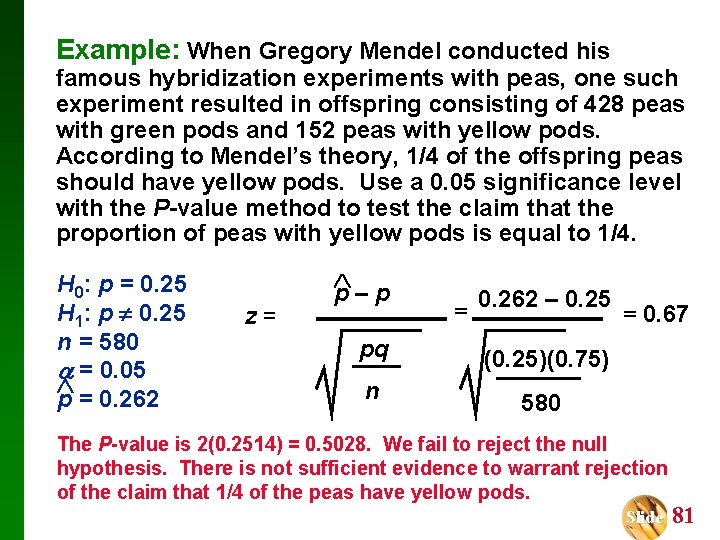
Example: When Gregory Mendel conducted his famous hybridization experiments with peas, one such experiment resulted in offspring consisting of 428 peas with green pods and 152 peas with yellow pods. According to Mendel’s theory, 1/4 of the offspring peas should have yellow pods. Use a 0. 05 significance level with the P-value method to test the claim that the proportion of peas with yellow pods is equal to 1/4. We note that n = 428 + 152 = 580, so p = 0. 262, and p = 0. 25. Slide 79

Example: When Gregory Mendel conducted his famous hybridization experiments with peas, one such experiment resulted in offspring consisting of 428 peas with green pods and 152 peas with yellow pods. According to Mendel’s theory, 1/4 of the offspring peas should have yellow pods. Use a 0. 05 significance level with the P-value method to test the claim that the proportion of peas with yellow pods is equal to 1/4. H 0: p = 0. 25 H 1: p 0. 25 n = 580 = 0. 05 p = 0. 262 z= p–p = 0. 262 – 0. 25 = 0. 67 pq (0. 25)(0. 75) n 580 Since this is a two-tailed test, the P-value is twice the area to the right of the test statistic. Using Table A-2, z = 0. 67 is 1 – 0. 7486 = 0. 2514. Slide 80

Example: When Gregory Mendel conducted his famous hybridization experiments with peas, one such experiment resulted in offspring consisting of 428 peas with green pods and 152 peas with yellow pods. According to Mendel’s theory, 1/4 of the offspring peas should have yellow pods. Use a 0. 05 significance level with the P-value method to test the claim that the proportion of peas with yellow pods is equal to 1/4. H 0: p = 0. 25 H 1: p 0. 25 n = 580 = 0. 05 p = 0. 262 z= p–p = 0. 262 – 0. 25 = 0. 67 pq (0. 25)(0. 75) n 580 The P-value is 2(0. 2514) = 0. 5028. We fail to reject the null hypothesis. There is not sufficient evidence to warrant rejection of the claim that 1/4 of the peas have yellow pods. Slide 81

Recap In this section we have discussed: v Test statistics for claims about a proportion. v P-value method. v Confidence interval method. v Obtaining p. Copyright © 2007 Pearson Education, Inc Publishing as Pearson Addison-Wesley. Slide 82

Section 8 -4 Testing a Claim About a Mean: Known Created by Erin Hodgess, Houston, Texas Revised to accompany 10 th Edition, Tom Wegleitner, Centreville, VA Slide 83

Key Concept This section presents methods for testing a claim about a population mean, given that the population standard deviation is a known value. This section uses the normal distribution with the same components of hypothesis tests that were introduced in Section 8 -2. Copyright © 2007 Pearson Education, Inc Publishing as Pearson Addison-Wesley. Slide 84

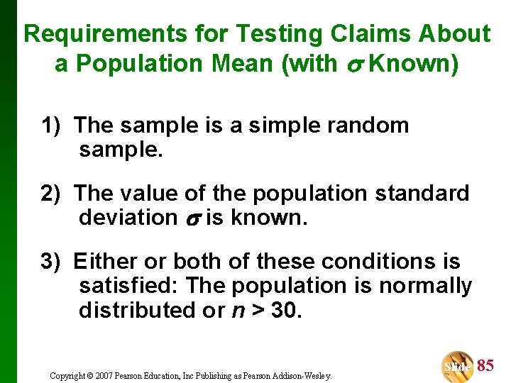
Requirements for Testing Claims About a Population Mean (with Known) 1) The sample is a simple random sample. 2) The value of the population standard deviation is known. 3) Either or both of these conditions is satisfied: The population is normally distributed or n > 30. Copyright © 2007 Pearson Education, Inc Publishing as Pearson Addison-Wesley. Slide 85

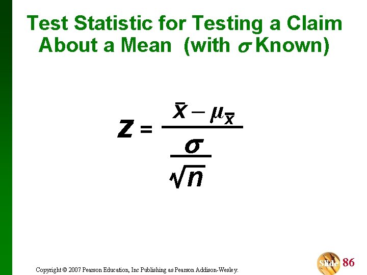
Test Statistic for Testing a Claim About a Mean (with Known) x – µx z = n Copyright © 2007 Pearson Education, Inc Publishing as Pearson Addison-Wesley. Slide 86

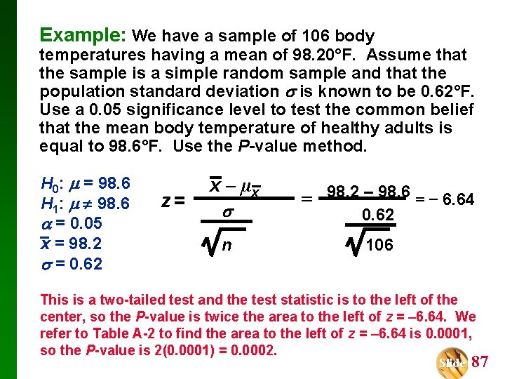
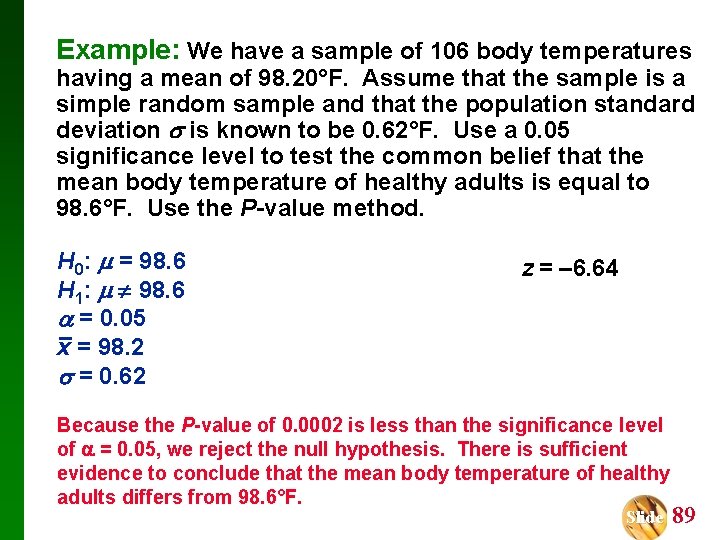
Example: We have a sample of 106 body temperatures having a mean of 98. 20°F. Assume that the sample is a simple random sample and that the population standard deviation is known to be 0. 62°F. Use a 0. 05 significance level to test the common belief that the mean body temperature of healthy adults is equal to 98. 6°F. Use the P-value method. H 0: = 98. 6 H 1: 98. 6 = 0. 05 x = 98. 2 = 0. 62 z = x – µx n = 98. 2 – 98. 6 = − 6. 64 0. 62 106 This is a two-tailed test and the test statistic is to the left of the center, so the P-value is twice the area to the left of z = – 6. 64. We refer to Table A-2 to find the area to the left of z = – 6. 64 is 0. 0001, so the P-value is 2(0. 0001) = 0. 0002. Slide 87

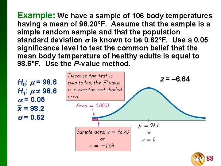
Example: We have a sample of 106 body temperatures having a mean of 98. 20°F. Assume that the sample is a simple random sample and that the population standard deviation is known to be 0. 62°F. Use a 0. 05 significance level to test the common belief that the mean body temperature of healthy adults is equal to 98. 6°F. Use the P-value method. H 0: = 98. 6 H 1: 98. 6 = 0. 05 x = 98. 2 = 0. 62 z = – 6. 64 Slide 88

Example: We have a sample of 106 body temperatures having a mean of 98. 20°F. Assume that the sample is a simple random sample and that the population standard deviation is known to be 0. 62°F. Use a 0. 05 significance level to test the common belief that the mean body temperature of healthy adults is equal to 98. 6°F. Use the P-value method. H 0: = 98. 6 H 1: 98. 6 = 0. 05 x = 98. 2 = 0. 62 z = – 6. 64 Because the P-value of 0. 0002 is less than the significance level of = 0. 05, we reject the null hypothesis. There is sufficient evidence to conclude that the mean body temperature of healthy adults differs from 98. 6°F. Slide 89

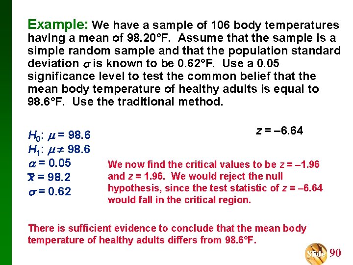
Example: We have a sample of 106 body temperatures having a mean of 98. 20°F. Assume that the sample is a simple random sample and that the population standard deviation is known to be 0. 62°F. Use a 0. 05 significance level to test the common belief that the mean body temperature of healthy adults is equal to 98. 6°F. Use the traditional method. H 0: = 98. 6 H 1: 98. 6 = 0. 05 x = 98. 2 = 0. 62 z = – 6. 64 We now find the critical values to be z = – 1. 96 and z = 1. 96. We would reject the null hypothesis, since the test statistic of z = – 6. 64 would fall in the critical region. There is sufficient evidence to conclude that the mean body temperature of healthy adults differs from 98. 6°F. Slide 90

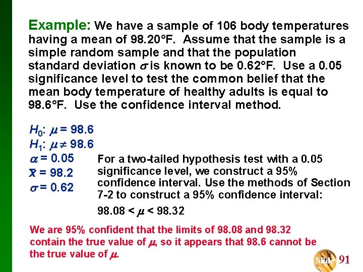
Example: We have a sample of 106 body temperatures having a mean of 98. 20°F. Assume that the sample is a simple random sample and that the population standard deviation is known to be 0. 62°F. Use a 0. 05 significance level to test the common belief that the mean body temperature of healthy adults is equal to 98. 6°F. Use the confidence interval method. H 0: = 98. 6 H 1: 98. 6 = 0. 05 For a two-tailed hypothesis test with a 0. 05 significance level, we construct a 95% x = 98. 2 confidence interval. Use the methods of Section = 0. 62 7 -2 to construct a 95% confidence interval: 98. 08 < < 98. 32 We are 95% confident that the limits of 98. 08 and 98. 32 contain the true value of , so it appears that 98. 6 cannot be the true value of . Slide 91

Underlying Rationale of Hypothesis Testing v If, under a given assumption, there is an extremely small probability of getting sample results at least as extreme as the results that were obtained, we conclude that the assumption is probably not correct. v When testing a claim, we make an assumption (null hypothesis) of equality. We then compare the assumption and the sample results and we form one of the following conclusions: Copyright © 2007 Pearson Education, Inc Publishing as Pearson Addison-Wesley. Slide 92

Underlying Rationale of Hypotheses Testing - cont v If the sample results (or more extreme results) can easily occur when the assumption (null hypothesis) is true, we attribute the relatively small discrepancy between the assumption and the sample results to chance. v If the sample results cannot easily occur when that assumption (null hypothesis) is true, we explain the relatively large discrepancy between the assumption and the sample results by concluding that the assumption is not true, so we reject the assumption. Copyright © 2007 Pearson Education, Inc Publishing as Pearson Addison-Wesley. Slide 93

Recap In this section we have discussed: v Requirements for testing claims about population means, σ known. v P-value method. v Traditional method. v Confidence interval method. v Rationale for hypothesis testing. Copyright © 2007 Pearson Education, Inc Publishing as Pearson Addison-Wesley. Slide 94

Section 8 -5 Testing a Claim About a Mean: Not Known Created by Erin Hodgess, Houston, Texas Revised to accompany 10 th Edition, Tom Wegleitner, Centreville, VA Slide 95

Key Concept This section presents methods for testing a claim about a population mean when we do not know the value of σ. The methods of this section use the Student t distribution introduced earlier. Copyright © 2007 Pearson Education, Inc Publishing as Pearson Addison-Wesley. Slide 96

Requirements for Testing Claims About a Population Mean (with Not Known) 1) The sample is a simple random sample. 2) The value of the population standard deviation is not known. 3) Either or both of these conditions is satisfied: The population is normally distributed or n > 30. Copyright © 2007 Pearson Education, Inc Publishing as Pearson Addison-Wesley. Slide 97

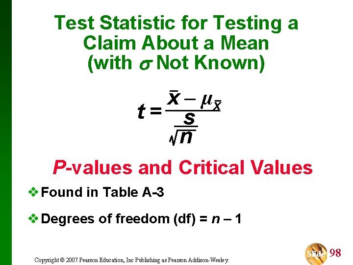
Test Statistic for Testing a Claim About a Mean (with Not Known) x – µx t= s n P-values and Critical Values v Found in Table A-3 v Degrees of freedom (df) = n – 1 Copyright © 2007 Pearson Education, Inc Publishing as Pearson Addison-Wesley. Slide 98

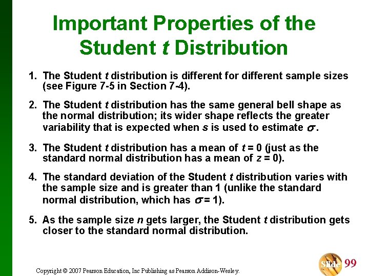
Important Properties of the Student t Distribution 1. The Student t distribution is different for different sample sizes (see Figure 7 -5 in Section 7 -4). 2. The Student t distribution has the same general bell shape as the normal distribution; its wider shape reflects the greater variability that is expected when s is used to estimate . 3. The Student t distribution has a mean of t = 0 (just as the standard normal distribution has a mean of z = 0). 4. The standard deviation of the Student t distribution varies with the sample size and is greater than 1 (unlike the standard normal distribution, which has = 1). 5. As the sample size n gets larger, the Student t distribution gets closer to the standard normal distribution. Copyright © 2007 Pearson Education, Inc Publishing as Pearson Addison-Wesley. Slide 99

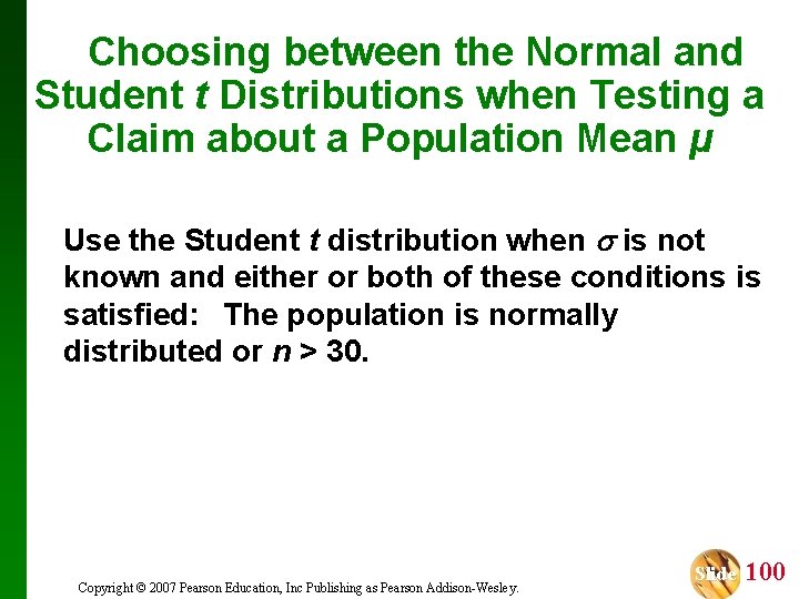
Choosing between the Normal and Student t Distributions when Testing a Claim about a Population Mean µ Use the Student t distribution when is not known and either or both of these conditions is satisfied: The population is normally distributed or n > 30. Copyright © 2007 Pearson Education, Inc Publishing as Pearson Addison-Wesley. Slide 100

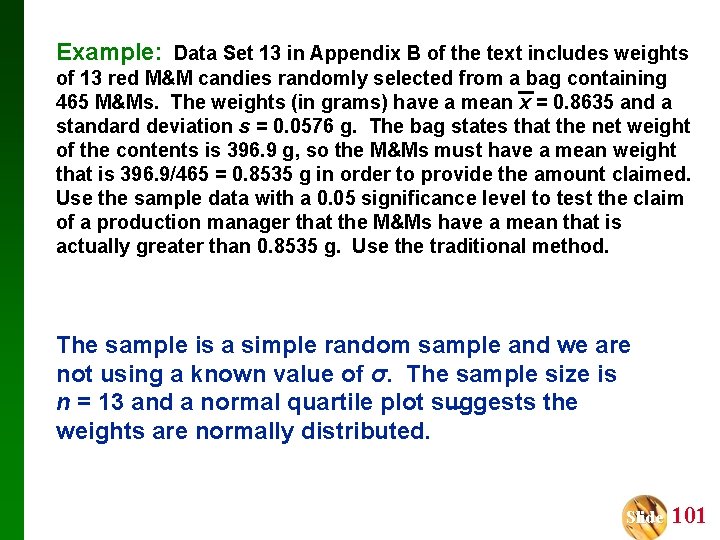
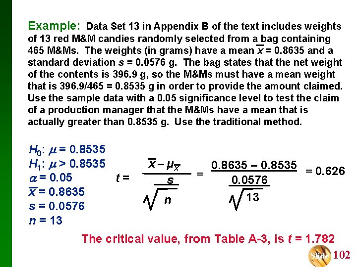
Example: Data Set 13 in Appendix B of the text includes weights of 13 red M&M candies randomly selected from a bag containing 465 M&Ms. The weights (in grams) have a mean x = 0. 8635 and a standard deviation s = 0. 0576 g. The bag states that the net weight of the contents is 396. 9 g, so the M&Ms must have a mean weight that is 396. 9/465 = 0. 8535 g in order to provide the amount claimed. Use the sample data with a 0. 05 significance level to test the claim of a production manager that the M&Ms have a mean that is actually greater than 0. 8535 g. Use the traditional method. The sample is a simple random sample and we are not using a known value of σ. The sample size is n = 13 and a normal quartile plot suggests the weights are normally distributed. Slide 101

Example: Data Set 13 in Appendix B of the text includes weights of 13 red M&M candies randomly selected from a bag containing 465 M&Ms. The weights (in grams) have a mean x = 0. 8635 and a standard deviation s = 0. 0576 g. The bag states that the net weight of the contents is 396. 9 g, so the M&Ms must have a mean weight that is 396. 9/465 = 0. 8535 g in order to provide the amount claimed. Use the sample data with a 0. 05 significance level to test the claim of a production manager that the M&Ms have a mean that is actually greater than 0. 8535 g. Use the traditional method. H 0: = 0. 8535 H 1: > 0. 8535 = 0. 05 t= x = 0. 8635 s = 0. 0576 n = 13 x – µx s n 0. 8635 – 0. 8535 = 0. 626 = 0. 0576 13 The critical value, from Table A-3, is t = 1. 782 Slide 102

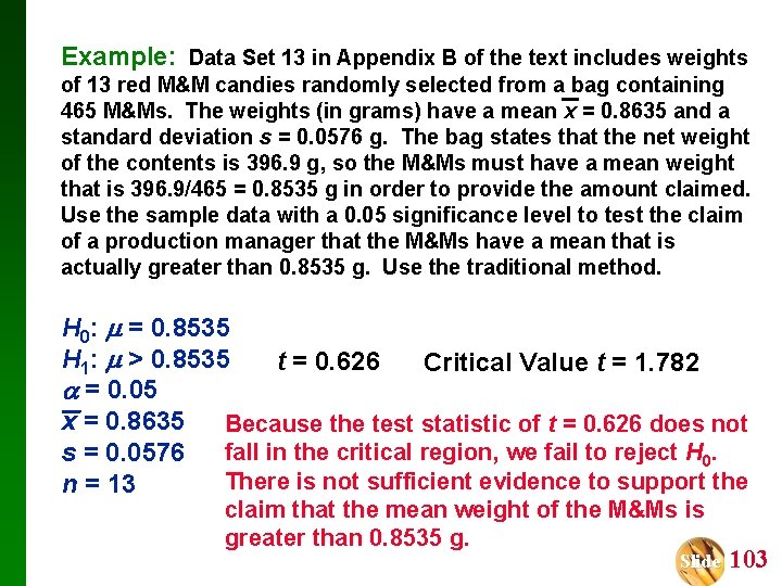
Example: Data Set 13 in Appendix B of the text includes weights of 13 red M&M candies randomly selected from a bag containing 465 M&Ms. The weights (in grams) have a mean x = 0. 8635 and a standard deviation s = 0. 0576 g. The bag states that the net weight of the contents is 396. 9 g, so the M&Ms must have a mean weight that is 396. 9/465 = 0. 8535 g in order to provide the amount claimed. Use the sample data with a 0. 05 significance level to test the claim of a production manager that the M&Ms have a mean that is actually greater than 0. 8535 g. Use the traditional method. H 0: = 0. 8535 H 1: > 0. 8535 t = 0. 626 Critical Value t = 1. 782 = 0. 05 x = 0. 8635 Because the test statistic of t = 0. 626 does not fall in the critical region, we fail to reject H 0. s = 0. 0576 There is not sufficient evidence to support the n = 13 claim that the mean weight of the M&Ms is greater than 0. 8535 g. Slide 103

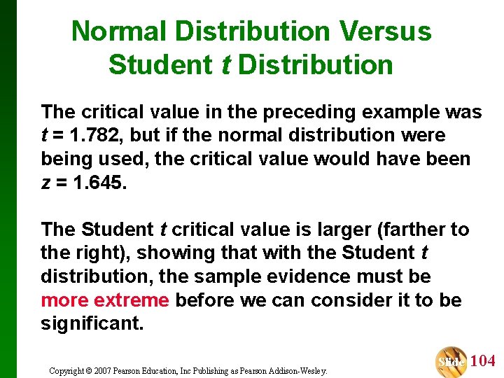
Normal Distribution Versus Student t Distribution The critical value in the preceding example was t = 1. 782, but if the normal distribution were being used, the critical value would have been z = 1. 645. The Student t critical value is larger (farther to the right), showing that with the Student t distribution, the sample evidence must be more extreme before we can consider it to be significant. Copyright © 2007 Pearson Education, Inc Publishing as Pearson Addison-Wesley. Slide 104

P-Value Method v Use software or a TI-83/84 Plus calculator. v If technology is not available, use Table A-3 to identify a range of P-values. Copyright © 2007 Pearson Education, Inc Publishing as Pearson Addison-Wesley. Slide 105

Example: Assuming that neither software nor a TI-83 Plus calculator is available, use Table A 3 to find a range of values for the P-value corresponding to the given results. a) In a left-tailed hypothesis test, the sample size is n = 12, and the test statistic is t = – 2. 007. b) In a right-tailed hypothesis test, the sample size is n = 12, and the test statistic is t = 1. 222. c) In a two-tailed hypothesis test, the sample size is n = 12, and the test statistic is t = – 3. 456. Slide 106

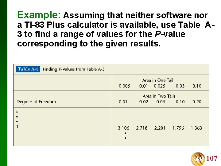
Example: Assuming that neither software nor a TI-83 Plus calculator is available, use Table A 3 to find a range of values for the P-value corresponding to the given results. Slide 107

Example: Assuming that neither software nor a TI-83 Plus calculator is available, use Table A -3 to find a range of values for the P-value corresponding to the given results. a) The test is a left-tailed test with test statistic t = – 2. 007, so the P-value is the area to the left of – 2. 007. Because of the symmetry of the t distribution, that is the same as the area to the right of +2. 007. Any test statistic between 2. 201 and 1. 796 has a right-tailed P- value that is between 0. 025 and 0. 05. We conclude that 0. 025 < P-value < 0. 05. Slide 108

Example: Assuming that neither software nor a TI-83 Plus calculator is available, use Table A -3 to find a range of values for the P-value corresponding to the given results. b) The test is a right-tailed test with test statistic t = 1. 222, so the P-value is the area to the right of 1. 222. Any test statistic less than 1. 363 has a right-tailed P-value that is greater than 0. 10. We conclude that P-value > 0. 10. Slide 109

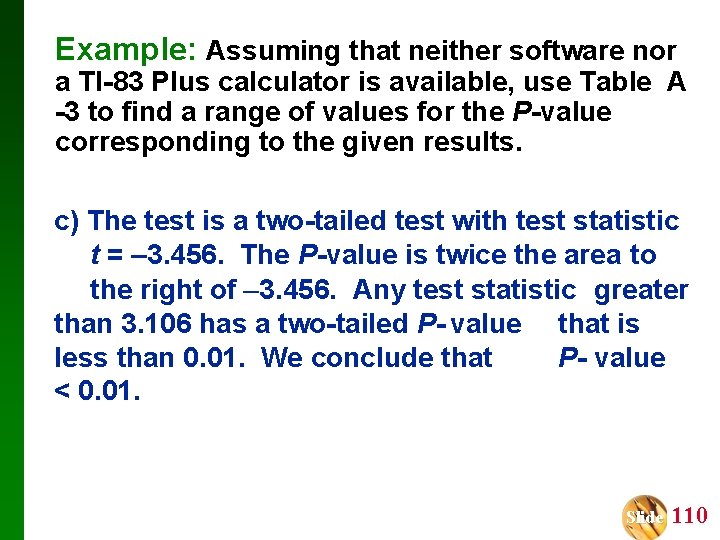
Example: Assuming that neither software nor a TI-83 Plus calculator is available, use Table A -3 to find a range of values for the P-value corresponding to the given results. c) The test is a two-tailed test with test statistic t = – 3. 456. The P-value is twice the area to the right of – 3. 456. Any test statistic greater than 3. 106 has a two-tailed P- value that is less than 0. 01. We conclude that P- value < 0. 01. Slide 110

Recap In this section we have discussed: v Assumptions for testing claims about population means, σ unknown. v Student t distribution. v P-value method. Copyright © 2007 Pearson Education, Inc Publishing as Pearson Addison-Wesley. Slide 111

Section 8 -6 Testing a Claim About a Standard Deviation or Variance Created by Erin Hodgess, Houston, Texas Revised to accompany 10 th Edition, Tom Wegleitner, Centreville, VA Slide 112

Key Concept This section introduces methods for testing a claim made about a population standard deviation σ or population variance σ 2. The methods of this section use the chi-square distribution that was first introduced in Section 7 -5. Copyright © 2007 Pearson Education, Inc Publishing as Pearson Addison-Wesley. Slide 113

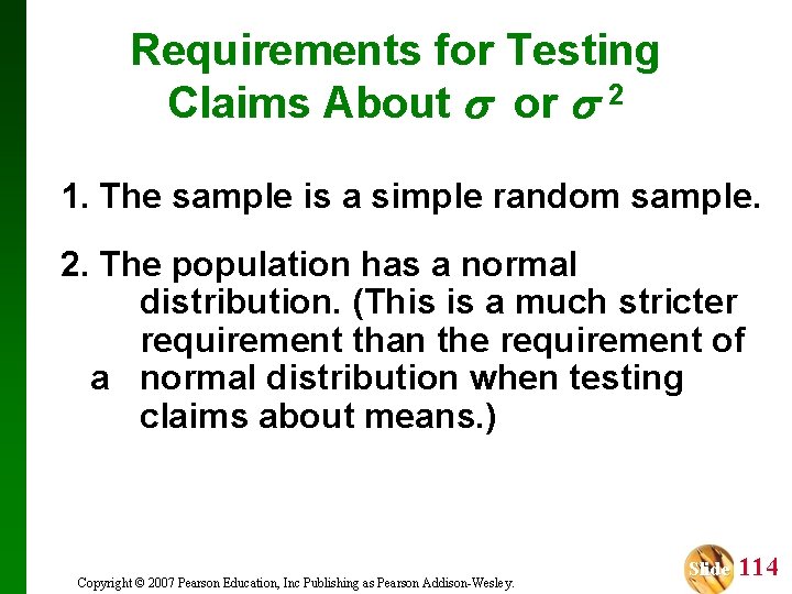
Requirements for Testing Claims About or 2 1. The sample is a simple random sample. 2. The population has a normal distribution. (This is a much stricter requirement than the requirement of a normal distribution when testing claims about means. ) Copyright © 2007 Pearson Education, Inc Publishing as Pearson Addison-Wesley. Slide 114

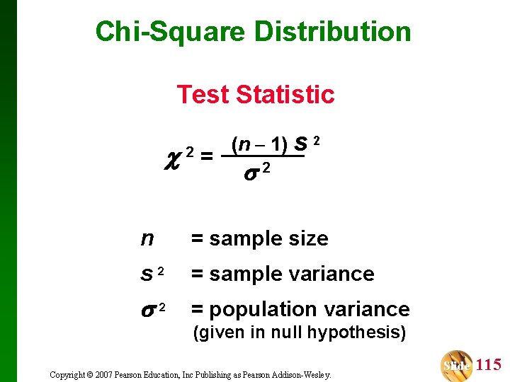
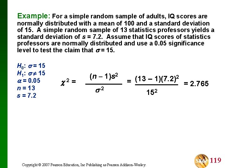
Chi-Square Distribution Test Statistic 2 = (n – 1) s 2 2 n = sample size s 2 = sample variance 2 = population variance (given in null hypothesis) Copyright © 2007 Pearson Education, Inc Publishing as Pearson Addison-Wesley. Slide 115

P-Values and Critical Values for Chi-Square Distribution v Use Table A-4. v The degrees of freedom = n – 1. Copyright © 2007 Pearson Education, Inc Publishing as Pearson Addison-Wesley. Slide 116

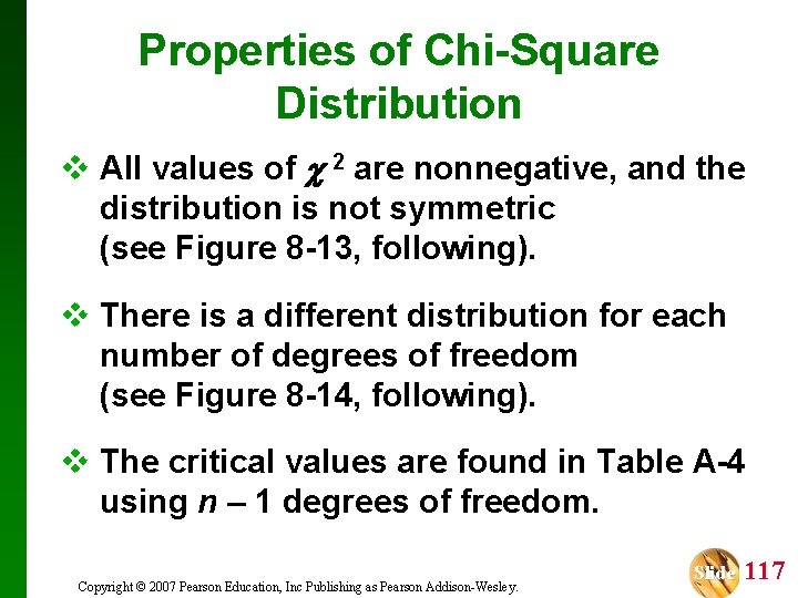
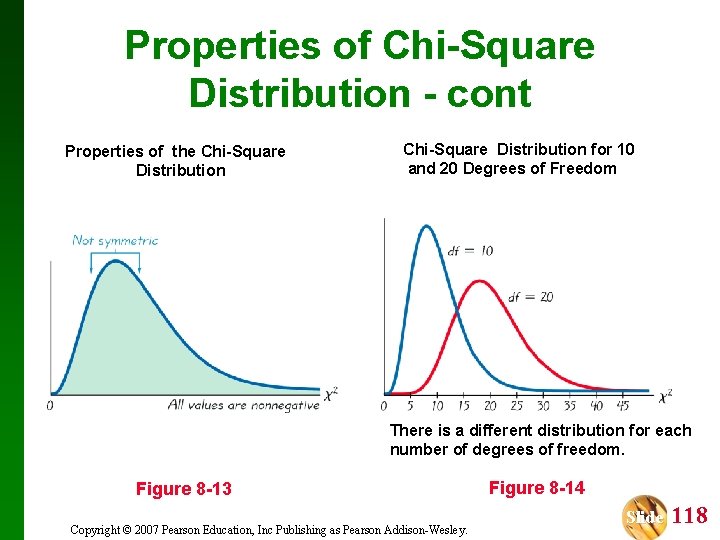
Properties of Chi-Square Distribution v All values of 2 are nonnegative, and the distribution is not symmetric (see Figure 8 -13, following). v There is a different distribution for each number of degrees of freedom (see Figure 8 -14, following). v The critical values are found in Table A-4 using n – 1 degrees of freedom. Copyright © 2007 Pearson Education, Inc Publishing as Pearson Addison-Wesley. Slide 117

Properties of Chi-Square Distribution - cont Properties of the Chi-Square Distribution Chi-Square Distribution for 10 and 20 Degrees of Freedom There is a different distribution for each number of degrees of freedom. Figure 8 -13 Copyright © 2007 Pearson Education, Inc Publishing as Pearson Addison-Wesley. Figure 8 -14 Slide 118

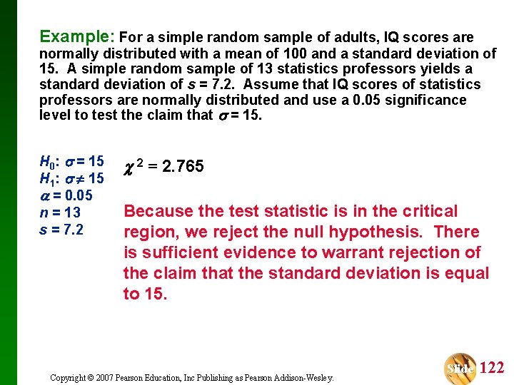
Example: For a simple random sample of adults, IQ scores are normally distributed with a mean of 100 and a standard deviation of 15. A simple random sample of 13 statistics professors yields a standard deviation of s = 7. 2. Assume that IQ scores of statistics professors are normally distributed and use a 0. 05 significance level to test the claim that = 15. H 0: = 15 H 1: 15 = 0. 05 n = 13 s = 7. 2 2 = (n – 1)s 2 2 2 (13 – 1)(7. 2) = = 2. 765 152 Copyright © 2007 Pearson Education, Inc Publishing as Pearson Addison-Wesley. Slide 119

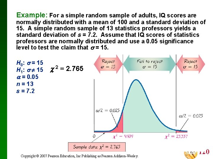
Example: For a simple random sample of adults, IQ scores are normally distributed with a mean of 100 and a standard deviation of 15. A simple random sample of 13 statistics professors yields a standard deviation of s = 7. 2. Assume that IQ scores of statistics professors are normally distributed and use a 0. 05 significance level to test the claim that = 15. H 0: = 15 H 1: 15 = 0. 05 n = 13 s = 7. 2 2 = 2. 765 Copyright © 2007 Pearson Education, Inc Publishing as Pearson Addison-Wesley. Slide 120

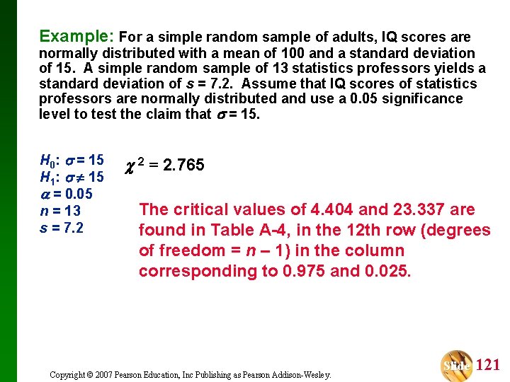
Example: For a simple random sample of adults, IQ scores are normally distributed with a mean of 100 and a standard deviation of 15. A simple random sample of 13 statistics professors yields a standard deviation of s = 7. 2. Assume that IQ scores of statistics professors are normally distributed and use a 0. 05 significance level to test the claim that = 15. H 0: = 15 H 1: 15 = 0. 05 n = 13 s = 7. 2 2 = 2. 765 The critical values of 4. 404 and 23. 337 are found in Table A-4, in the 12 th row (degrees of freedom = n – 1) in the column corresponding to 0. 975 and 0. 025. Copyright © 2007 Pearson Education, Inc Publishing as Pearson Addison-Wesley. Slide 121

Example: For a simple random sample of adults, IQ scores are normally distributed with a mean of 100 and a standard deviation of 15. A simple random sample of 13 statistics professors yields a standard deviation of s = 7. 2. Assume that IQ scores of statistics professors are normally distributed and use a 0. 05 significance level to test the claim that = 15. H 0: = 15 H 1: 15 = 0. 05 n = 13 s = 7. 2 2 = 2. 765 Because the test statistic is in the critical region, we reject the null hypothesis. There is sufficient evidence to warrant rejection of the claim that the standard deviation is equal to 15. Copyright © 2007 Pearson Education, Inc Publishing as Pearson Addison-Wesley. Slide 122

Recap In this section we have discussed: v Tests for claims about standard deviation and variance. v Test statistic. v Chi-square distribution. v Critical values. Copyright © 2007 Pearson Education, Inc Publishing as Pearson Addison-Wesley. Slide 123